


ICML 2015. [Paper] [Github]
Jascha Sohl-Dickstein, Eric A. Weiss, Niru Maheswaranathan, Surya Ganguli
Stanford University | University of California, Berkeley
12 Mar 2015
Introduction
Generative models trade-off between tractability and flexibility. A tractable model is numerically computed, such as a Gaussian distribution, and can be easily fitted to the data. However, these models are difficult to adequately describe complex datasets. Conversely, flexible models can adequately describe arbitrary data, but typically require very complex Monte Carlo processes to train, evaluate, and generate samples.
The authors propose a new way to define a probabilistic model with four possibilities:
- Extremely flexible model structure
- Accurate sampling
- Easy multiplication with other distributions for post-computation etc.
- It is easy to calculate the model log likelihood and the probability of each state
The author uses a generative Markov chain that gradually transforms from a well-known distribution, such as the Gaussian distribution, to the distribution of the target data using a diffusion process. Since it is a Markov chain, each state is independent of the previous state. Since the probability of each step in the diffusion chain can be calculated numerically, the entire chain can also be calculated numerically.
Estimating small changes to the diffusion process is involved in the learning process. This is because it is more tractable to estimate small changes than to describe the entire distribution using one potential function that cannot be numerically normalized. In addition, since a diffusion process exists for any data distribution, this method can express any type of data distribution.
Algorithms
The goal of this thesis is to define a forward diffusion process that transforms any complex data distribution into a simple and tractable distribution, and learn a finite-time inverse transformation process. This inverse transformation process is a targeted generative model because it transforms a simple distribution into a target data distribution. The paper also derives the entropy bounds of the inverse transformation process and shows how a learned distribution can be multiplied with another distribution.
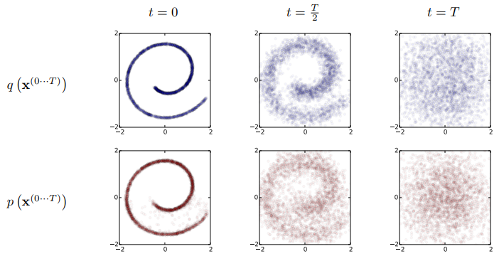
1. Forward Trajectory
$q(x^{(0)})$ for data distribution, $\pi(y)$ for tractable simple distribution, $T_\pi (y | y) for Markov diffusion kernel for $\pi(y)$ ‘)$, if the diffusion rate is $\beta$, it is as follows.
\[\begin{equation} \pi(y) = \int dy' T_\pi (y | y'; \beta) \pi(y') \\ q(x^{(t)} | x^{(t-1)}) = T_\pi (x^{(t)} | x^{(t-1)} ; \beta _t) \end{equation}\]
If diffusion is performed in the $T$ step in the data distribution $q(x^{(0)})$, it is as follows.
$q(x^{(t)}|x^{(t-1)})$ is either a Gaussian distribution with equal variance or an independent binomial distribution.
2. Reverse Trajectory
Reverse trajectory is the same trajectory as forward trajectory, but is trained to proceed in reverse.
\[\begin{equation} p(x^{(T)}) = \pi (x^{(T)}) \\ p(x^{(0 \cdots T)}) = p(x^{(T)}) \prod_{t=1}^T p(x^{(t-1)} | x^{(t )}) \end{equation}\]For continuous diffusion, reverse must be in the same functional form as forward. If $q(x^{(t)}|x^{(t-1)})$ is a Gaussian distribution and $\beta_t$ is small then $q(x^{(t-1)}|x^{( t)})$ is also a Gaussian distribution. The longer the trajectory, the smaller the diffusion rate $\beta$ can be.
In the learning process, we only need to predict the mean and variance of the Gaussian distribution kernel. The computational cost of this algorithm is the product of the cost of the function of mean and variance and the number of time-steps. In all experiments in the paper, these functions are MLPs.
3. Model Probability
The probability of the generative model for the data distribution is:
\[\begin{equation} p(x^{(0)}) = \int dx^{(1 \cdots T)} p(x^{(0 \cdots T)}) \end{equation}\]This integral is not tractable. So instead we compute the relative probabilities of forward and reverse averaged over forwards. (It is said to have been inspired by Annealed importance sampling and the Jarzynski equation)
\[\begin{aligned} p(x^{(0)}) &= \int dx^{(1 \cdots T)} p(x^{(0 \cdots T)}) \frac{q(x^{(1 \cdots T)} | x^{(0)})}{q(x^{(1 \cdots T)} | x^{(0)})} \\ &= \int dx^{(1 \cdots T)} q(x^{(1 \cdots T)} | x^{(0)}) \frac{p(x^{(0 \cdots T)})}{q(x^{(1 \cdots T)} | x^{(0)})} \\ &= \int dx^{(1 \cdots T)} q(x^{(1 \cdots T)} | x^{(0)}) p(x^{(T)}) \prod_{t=1}^T \frac{p(x^{(t-1)}|x^{(t)})}{q(x^{(t)} | x^{(t- One)})} \end{aligned}\]4. Training
Learning proceeds in the direction of maximizing the model log likelihood.
\[\begin{aligned} L &= \int dx^{(0)} q(x^{(0)}) \log p(x^{(0)}) \\ &= \int dx^{(0)} q(x^{(0)}) \log \bigg[ \int dx^{(1 \cdots T)} q(x^{(1 \cdots T)} | x^{(0)}) p(x^{(T)}) \prod_{t=1}^T \frac{p(x^{(t-1)}|x^{(t)})}{q(x^{(t)} | x^{(t-1)})} \bigg] \end{aligned}\]According to Jensen’s inequality, $L$ has a lower bound.
\[\begin{aligned} L &\ge \int dx^{(0 \cdots T)} q(x^{(0 \cdots T)}) \log \bigg[ p(x^{(T)}) \prod_{t=1}^T \frac{p(x^{(t-1)}|x^{(t)})}{q(x^{( t)} | x^{(t-1)})} \bigg] = K \end{aligned}\]By Appendix, $K$ can be expressed with KL divergence and entropy as follows.
\[\begin{aligned} L \ge K =& -\sum_{t=2}^T \int dx^{(0)} dx^{(t)} q(x^{(0)}, x^{(t)}) D_{KL} \bigg( q(x^{(t-1)} | x^{(t)}, x^{(0)}) \; || \; p(x^{(t-1)} | x^{(t)}) \bigg) \\ &+ H_q (X^{(T)} | X^{(0)}) - H_q (X^{(1)} | X^{(0)}) - H_p (X^{(T)}) \end{aligned}\]Since entropies and KL divergence are computable, $K$ is computable. The equal sign holds when forward and reverse are equal, so if $\beta_t$ is sufficiently small, $L$ is almost equal to $K$.
Learning to find the reverse Markov transition is equivalent to maximizing the lower bound.
\[\begin{aligned} \hat{p} (x^{(t-1)} | x^{(t)}) = \underset{p(x^{(t-1)} | x^{(t)})}{ \operatorname{argmax}} K \end{aligned}\]How you choose $\beta_t$ is important to the model’s performance. In the case of the Gaussian distribution, $\beta_{2 \cdots T}$ was obtained by gradient ascent for $K$, and $\beta_1$ was said to be a fixed value to prevent overfitting.
5. Multiplying Distributions, and Computing Posteriors
A new distribution is obtained by multiplying the model’s distribution p(x^{(0)}) by another distribution r(x^{(0)}) Let’s say we create $\tilde{p}(x^{(0)}) \propto p(x^{(0)}) r(x^{(0)})$. For each distribution $p(x^{(t)})$ and $r(x^{(t)}) in $t$ to find $\tilde{p}(x^{(0)})$ Multiply by $ to get $\tilde{p}(x^{(t)})$, and think of $\tilde{p}(x^{(0 \cdots T)})$ as a modified reverse trajectory. Since $\tilde{p}$ is also a probability distribution, it can be defined using the normalizing constant $\tilde{Z}_t$.
\[\begin{equation} \tilde{p} (x^{(t)}) = \frac{1}{\tilde{Z}_t} p(x^{(t)}) r(x^{(t)}) \end{equation}\]
The Markov kernel $p(x^{(t)} | x^{(t+1)})$ of the reverse diffusion process follows the equation:
If Pertubed Markov kernel $\tilde{p}(x^{(t)} | x^{(t+1)})$ also follows the above formula, then
Therefore, the following equation holds.
\[\begin{equation} \tilde{p} (x^{(t)} | x^{(t+1)}) = p (x^{(t)} | x^{(t+1)}) \frac{\tilde{Z}_{t+1} r(x^{(t)})}{\tilde{Z}_t r(x^{(t+1)})} \end{equation}\]Since the above expression may not be a normalized probability distribution, we define it as
\[\begin{equation} \tilde{p} (x^{(t)} | x^{(t+1)}) = \frac{1}{\tilde{Z}_t (x^{(t+1)})} p (x^{(t)} | x^{(t+1)}) r(x^{(t)}) \end{equation}\]
In the case of Gaussian distribution, it is said that each diffusion step has a peak at $r(x^{(t)})$ due to small variance. This translates $\frac{r(x^{(t)})}{r(x^{(t+1)})}$ into $p(x^{(t)} | x^{(t+1 )})$ can be thought of as a small pertubation. Since a small pertubation of the Gaussian distribution affects the mean but not the normalization constant, it can be defined as the above equation.
If r(x^{(t)}) is sufficiently smooth, it can be considered as a small pertubation of the reverse diffusion kernel p(x^{(t)}|x^{(t+1)})$. In this case, $\tilde{p}$ has the same form as $p$. If $r(x^{(t)})$ can be multiplied by Gaussian distribution and closed form then $r(x^{(t)})$ is $p(x^{(t)}|x^{ (t+1)})$ can be multiplied by closed from.
$r(x^{(t)})$ should be chosen as a function that changes slowly along the trajectory and was kept constant in the experiment.
Since we know the forward, we can find the upper and lower bounds for the conditional entropy of each step in reverse, so we can get the log likelihood.
\[\begin{equation} H_q (X^{(t)}|X^{(t-1)}) + H_q (X^{(t-1)}|X^{(0)}) - H_q (X^{(t) }|X^{(0)}) \le H_q (X^{(t-1) }|X^{(t)}) \le H_q (X^{(t)}|X^{(t-1) One)}) \end{equation}\]
The upper and lower bounds depend only on $q(x^{(1 \cdots T)}|x^{(0)})$ so they can be computed.
Experiments
- Dataset: Toy data, MNIST, CIFAR10, Dead Leaf Images, Bark Texture Images
- Creation and impainting for each dataset
Forward diffusion kernel and reverse diffusion kernel are as follows.
\[\begin{equation} q(x^{(t)}|x^{(t-1)}) = \mathcal{N} (x^{(t)}; x^{(t-1)} \sqrt{1-\beta_t}, I \beta_t) \\ p(x^{(t-1)}|x^{(t)}) = \mathcal{N} (x^{(t-1)}; f_\mu (x^{(t)}, t), f_\Sigma (x^{(t)}, t)) \end{equation}\]$f_\mu$ and $f_\Sigma$ are MLPs, and $f_\mu$, $f_\Sigma$, and $\beta_{1 \cdots T}$ are learning targets.
Results

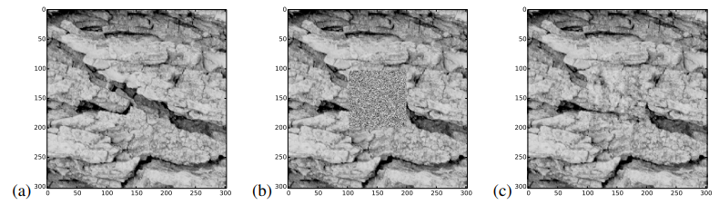
It’s a little different from the original, but it turned out to be quite good.
![[Paper review] Self-correcting LLM-controlled Diffusion Models](/assets/images/blog/post-5.jpg)