Blogs

arXiv 2023. [Paper] [Page]
Shengming Yin, Chenfei Wu, Huan Yang, Jianfeng Wang, Xiaodong Wang, Minheng Ni, Zhengyuan Yang, Linjie Li, Shuguang Liu, Fan Yang, Jianlong Fu, Gong Ming, Lijuan Wang, Zicheng Liu, Houqiang Li, Nan Duan
University of Science and Technology of China | Microsoft Research Asia | Microsoft Azure AI
22 Mar 2023

Introduction

Many previous studies have demonstrated the ability to generate high-definition images and short videos. However, videos in real applications are often much longer than 5 seconds. Movies typically last 90 minutes or more, and cartoons are usually 30 minutes long. Even for “short” video applications like TikTok, the recommended video length is 21-34 seconds. Creating longer videos is becoming increasingly important as the demand for engaging visual content continues to grow.

However, scaling it up to create long movies presents significant challenges as it requires large amounts of computational resources. To overcome this problem, most modern approaches use an “Autoregressive over X” architecture. Here, “X” represents all creation models capable of creating short movie clips, including autoregressive models such as Phenaki, TATS, and NUWA-Infinity, and diffusion models such as MCVD, FDM, and LVDM. The basic idea of this approach is to train a model with short movie clips and then use them to generate longer movies with a sliding window during inference. The “Autoregressive over X” architecture not only greatly reduces the computational burden, but also eases the data requirements for long videos as only short videos are required for training.

Unfortunately, while the “Autoregressive over X” architecture is a resourceful solution for generating long videos, it introduces new difficulties.

1. Unrealistic shot changes and long-term discrepancies can occur in the long videos generated because the model doesn’t have a chance to learn these patterns from the long videos.
2. Due to the sliding window’s dependency limitations, the inference process cannot be performed in parallel, so it takes much more time.

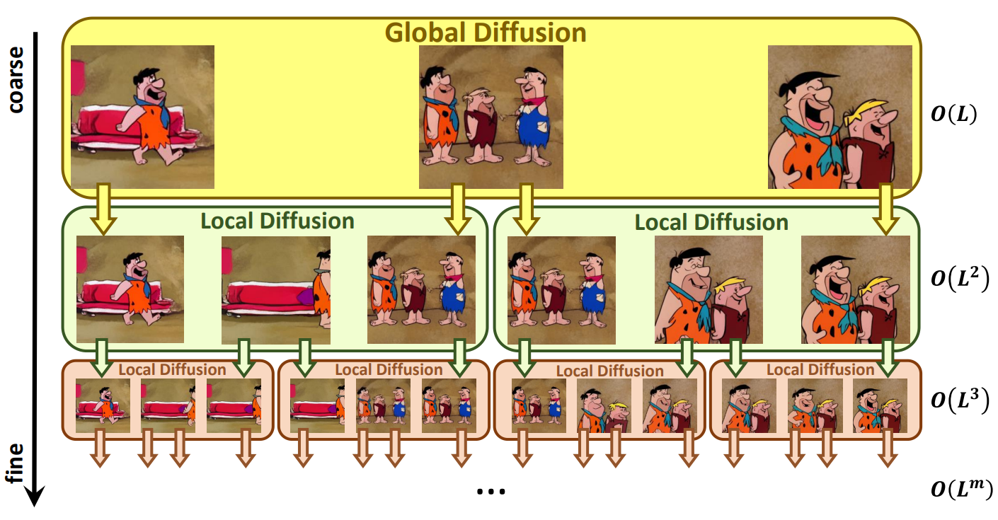
In order to solve the above problem, this paper proposes a “Diffusion over Diffusion” architecture, NUWA-XL, which creates a long video with a “coarse-to-fine” process as shown in the figure above. First, the global diffusion model generates $L$ keyframes based on $L$ prompts, and these keyframes form the rough storyline of the video. The first local diffusion model treats $L$ prompts and adjacent keyframes as the first and last frames, respectively, and creates $L-2$ intermediate frames, totaling $L + (L-1)\times(L -2) Create \approx L^2$ detailed frames.

If you repeatedly apply local diffusion to fill the middle frame, the length of the video increases exponentially, resulting in a very long video. For example, a NUWA-XL with a depth of $m$ and a local diffusion length of $L$ can create a long movie with a size of $O(L^m)$. The advantages of this approach are threefold.

1. This hierarchical architecture allows the model to learn directly from long videos, eliminating the mismatch between training and inference.
2. It naturally supports parallel inference, so it can greatly improve the inference speed when creating long movies.
3. It can easily scale to longer videos because the length of a video can grow exponentially.

Method

1. Temporal KLVAE (T-KLVAE)

Learning and sampling the diffusion model directly from pixels is computationally expensive. KLVAE compresses the original image into a low-dimensional latent representation that can alleviate this problem by performing a diffusion process. To utilize the external knowledge of pretrained image KLVAE and transfer it to video, the authors propose Temporal KLVAE (T-KLVAE) by adding an external temporal convolution and attention layer while retaining the original spatial module.

Video $v \in \mathbb{R}^{b \times L \ Given times C \times H \times W}$, it is first viewed as $L$ independent images and encoded with pretrained KLVAE spatial convolution. We add a temporal convolution after each spatial convolution to further model temporal information. To keep the original pretrained knowledge intact, the temporal convolution is initialized with an identity function that guarantees exactly the same output as the original KLVAE.

Specifically, the convolution weight $W^{conv1d} \in \mathbb{R}^{c_{out} \times c_{in} \times k}$ is first set to 0. Here, $c_{out}$ represents the output channel, $c_{in}$ represents the input channel and is the same as $c_{out}$, and $k$ represents the size of the temporal kernel. Then, for each output channel $i$, the middle $(k - 1)//2$ of the kernel size of the corresponding input channel $i$ is set to 1.

\[\begin{equation} W^{conv1d}[i, i, (k-1)//2] = 1 \end{equation}\]

Similarly, we add temporal attention after the original spatial attention and initialize the output projection layer’s weight $W^\textrm{att_out}$ to 0.

\[\begin{equation} W^\textrm{att_out} = 0 \end{equation}\]

For the T-KLVAE decoder $D$, the same initialization strategy is used. The objective function of T-KLVAE is the same as image KLVAE. Finally, we get the latent code $x_0 \in \mathbb{R}^{b \times L \times c \times h \times w}$, which is a compact representation of the original video $v$.

2. Mask Temporal Diffusion (MTD)

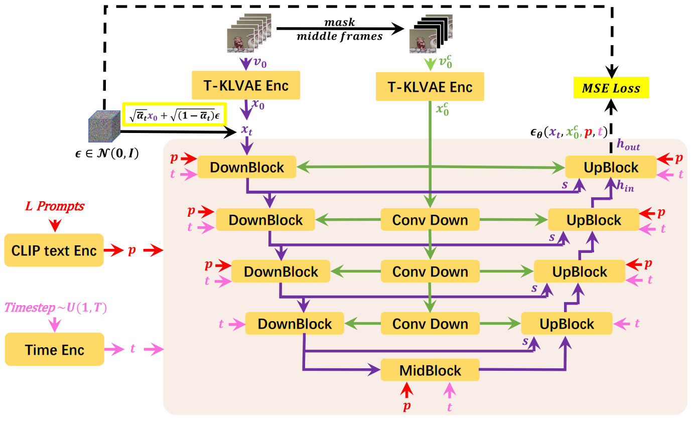
Next, Mask Temporal Diffusion (MTD) is introduced as the basic diffusion model of the proposed Diffusion over Diffusion architecture. In the case of global diffusion, only $L$ prompts are used as inputs to form the approximate storyline of the video, but in the case of local diffusion, the input consists of the first and last frames as well as $L$ prompts. The proposed MTD, which can accommodate input conditions with or without the first frame and the last frame, supports both global and local diffusion.

First, $L$ prompt inputs are embedded into CLIP Text Encoder to obtain prompt embedding $p \in \mathbb{R}^{b \times L \times l_p \times d_p}$. Here, $b$ is the batch size, $l_p$ is the number of tokens, and $d_p$ is the dimension of the prompt embedding. The randomly sampled diffusion timestep $t \in U(1, T)$ is embedded with the timestep embedding $t \in \mathbb{R}^c$. The video $v_0 \in \mathbb{R}^{b \times L \times C \times H \times W}$ is encoded in T-KLVAE and $x_0 \in \mathbb{R}^{b \times L \ get times c \times h \times w}$

According to the predefined diffusion process, $x_0$ is damaged as follows.

\[\begin{equation} q(x_t \vert x_{t-1}) = \mathcal{N}(x_t; \sqrt{\alpha_t} x_{t-1}, (1-\alpha_t) I) \end{equation}\] \[\begin{equation} x_t = \sqrt{\vphantom{1} \bar{\alpha}_t} x_0 + (1 - \bar{\alpha}_t) \epsilon, \quad \epsilon \sim \mathcal{N}(0,I) \end{equation}\]

where $\epsilon \in \mathbb{R}^{b \times L \times c \times h \times w}$ is noise, and $x_t \in \mathbb{R}^{b \times L \times c \times h \times w}$ is the tth intermediate state of the diffusion process.

In the case of the global diffusion model, the visual condition $v_0^c$ is all zero. On the other hand, for the local diffusion model, $v_0 \in \mathbb{R}^{b \times L \times C \times H \times W}$ is obtained by masking the middle $L-2$ frame of $v_0$. can $v_0^c$ is also encoded with T-KLVAE to get $x_0^c \in \mathbb{R}^{b \times L \times c \times h \times w}$.

Finally, $x_t$, $p$, $t$, and $x_0^c$ are entered into Mask 3D-UNet $\epsilon_\theta (\cdot)$. Then the model is the output of Mask 3D-UNet $\epsilon_\theta (x_t, p, t, x_0^c) \in \mathbb{R}^{b \times L \times c \times h \times w}$ Minimize the distance between $\epsilon$ and $\epsilon$.

\[\begin{equation} \mathcal{L}_\theta = \|\epsilon - \epsilon_\theta(x_t, p, t, x_0^c)\|_2^2 \end{equation}\]

While Mask 3D-UNet is composed of multi-scale DownBlocks and UpBlocks with skip connection, $x_0^c$ is downsampled to the corresponding resolution using the cascade of the convolution layer and supplied to the corresponding DownBlock and UpBlock.

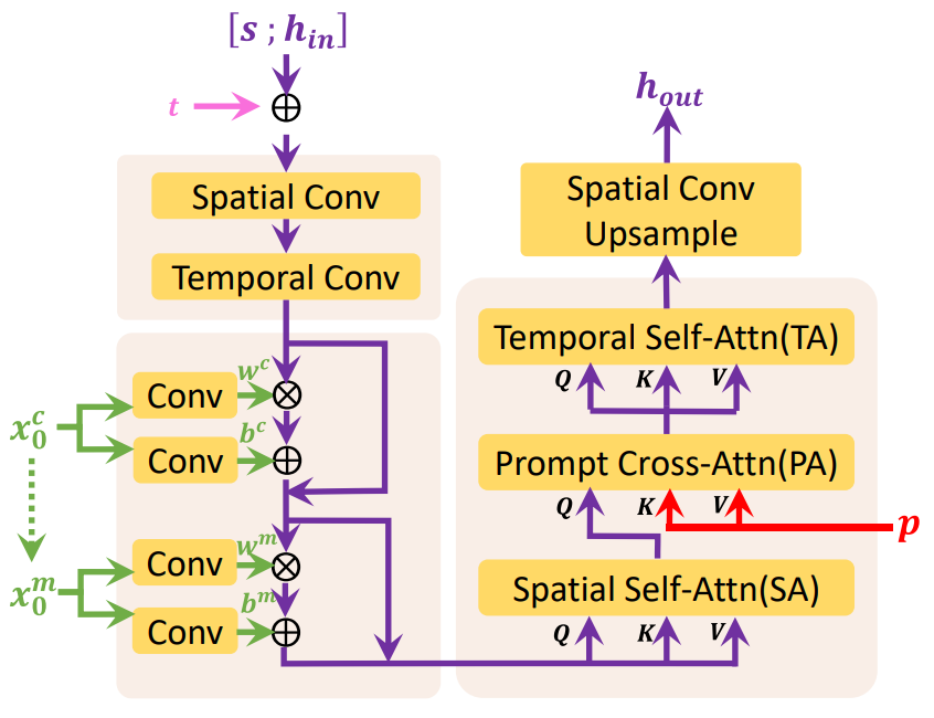
The picture above shows the details of the last UpBlock of Mask 3D-UNet. UpBlock receives hidden state $h_in$, skip connection $s$, timestep embedding $t$, visual condition $x_0^c$, and prompt embedding $p$ as inputs and outputs hidden state $h_out$. In the case of global diffusion, $x_0^c$ does not contain valid information because there is no frame provided as a condition, but in the case of local diffusion, $x_0^c$ includes the encoded information of the first frame and the last frame.

$s \in \mathbb{R}^{b \times L \times c_{skip} \times h \times w}$ first $h_{in} \in \mathbb{R}^{b \times L \ concat with times c_{in} \times h \times w}$.

\[\begin{equation} h := [s; h_{in}] \in \mathbb{R}^{b \times L \times (c_{skip} + c_{in}) \times h \times w} \end{equation}\]

$h$ becomes $h \in \mathbb{R}^{b \times L \times c \times h \times w}$ through convolution operation. Then $t$ is added to $h$ as a channel dimension.

\[\begin{equation} h := h + t \end{equation}\]

To exploit the external knowledge of the pretrained text-to-image model, factorized convolution and attention are introduced, the spatial layer is initialized with pretrained weights and the temporal layer is initialized with the identity function.

For spatial convolution, $L$ is treated as the batch size, resulting in $h \in \mathbb{R}^{(b \times L) \times c \times h \times w}$, and for temporal convolution, spatial Axis $hw$ is treated as batch size, resulting in $h \in \mathbb{R}^{(b \times hw) \times c \times L}$.

\[\begin{aligned} h &:= \textrm{SpatialConv}(h) \\ h &:= \textrm{TemporalConv}(h) \end{aligned}\]

Then $h$ is conditioned by $x_0^c$ and $x_0^m$, and $x_0^m$ is a binary mask indicating which frame is conditioned. $x_0^c$ and $x_0^m$ are first converted to scale $w^c$, $w^m$ and shift $b^c$, $b^m$ by the convolution layer initialized to 0. It is then injected into $h$ as a linear projection.

\[\begin{aligned} h &:= w^c \cdot h + b^c + h \\ h &:= w^m \cdot h + b^m + h \end{aligned}\]

Then, Spatial Self-Attention (SA), Prompt Cross-Attention (PA), and Temporal Self-Attention (TA) are sequentially applied to $h$.

For SA, $h$ is reshaped to $h \in \mathbb{R}^{(b \times L) \times hw \times c}$.

\[\begin{equation} Q^{SA} = hW_Q^{SA}, \quad K^{SA} = hW_K^{SA}, \quad V^{SA} = hW_V^{SA} \\ \tilde{Q}^{SA} = \textrm{Selfattn} (Q^{SA}, K^{SA}, V^{SA}) \end{equation}\]

$W_Q^{SA}, W_K^{SA}, W_V^{SA} \in \mathbb{R}^{c \times d_{in}}$ are the learned parameters.

For PA, $p$ is reshaped to $p \in \mathbb{R}^{(b \times L) \times l_p \times d_p}$.

\[\begin{equation} Q^{PA} = hW_Q^{PA}, \quad K^{PA} = pW_K^{PA}, \quad V^{PA} = pW_V^{PA} \\ \tilde{Q}^{SA} = \textrm{Crossattn} (Q^{PA}, K^{PA}, V^{PA}) \end{equation}\]

$W_Q^{PA} \in \mathbb{R}^{c \times d_{in}}$, $W_K^{PA}, W_V^{PA} \in \mathbb{R}^{d_p \times d_ {in}}$ is the parameter to be learned.

TA is the same as SA, except that the spatial axis $hw$ is treated as the batch size and $L$ is treated as the sequence length.

Finally, $h$ is upsampled to the target resolution $h_{out} \in \mathbb{R}^{b \times L \times c \times h_{out} \times h_{out}}$ through spatial convolution. do. Likewise, the other blocks of Mask 3D-UNet utilize the same structure to process their inputs.

3. Diffusion over Diffusion Architecture

In the inference step, given $L$ prompts $p$ and visual condition $v_0^c$, $x_0$ is sampled from pure noise $x_T$ by MTD. Specifically, for each timestep $t = T, T − 1, \cdots, 1$, the intermediate state $x_t$ in the diffusion process is updated as follows.

\[\begin{equation} x_{t-1} = \frac{1}{\sqrt{\alpha}_t} \bigg( x_t - \frac{1 - \alpha_t}{\sqrt{1 - \bar{\alpha}_t}} \epsilon_\theta (x_t, p, t, x_0^c) \bigg) + \frac{(1 - \bar{\alpha}_{t-1}) \beta_t}{1 - \bar{\alpha}_t} \epsilon \end{equation}\]

Finally, the sampled latent code $x_0$ is decoded into video pixel $v_0$ by T-KLVAE. For simplicity, the MTD’s iterative creation process is shown as follows.

\[\begin{equation} v_0 = \textrm{Diffusion} (p, v_0^c) \end{equation}\]

When creating a long video, if $L$ number of prompts $p_1$ are given at large intervals, $L$ keyframes are first created through the global diffusion model.

\[\begin{equation} v_{01} = \textrm{GlobalDiffusion} (p_1, v_{01}^c) \end{equation}\]

Here, $v_{01}^c$ is all 0. Temporarily sparse keyframe $v_{01}$ forms a rough storyline of the video.

Then adjacent keyframes in $v_{01}$ are treated as first and last frames in visual condition $v_{02}^c$. The middle $L-2$ frames are generated by supplying $p_2$ and $v_{02}^c$ to the first local diffusion model. Here, $p_2$ is $L$ prompts with shorter time intervals.

\[\begin{equation} v_{02} = \textrm{LocalDiffusion} (p_2, v_{02}^c) \end{equation}\]

Similarly, $v_{03}^c$ can be obtained from adjacent frames of $v_{02}$, and $p_3$ is $L$ prompts with a shorter time interval than $p_2$. $p_3$ and $v_{03}^c$ are supplied to the second local diffusion model.

\[\begin{equation} v_{03} = \textrm{LocalDiffusion} (p_3, v_{03}^c) \end{equation}\]

Compared to the frames of $v_{01}$, the frames of $v_{02}$ and $v_{03}$ are finer with more details and strong consistency.

By repeatedly applying local diffusion to complete the middle frame, a model with a depth of $m$ can create a very long movie with a length of $O(L^m)$. Meanwhile, through this hierarchical architecture, it is possible to eliminate the gap between learning and inference by directly learning temporally sparsely sampled frames from a long video (3376 frames). After sampling $L$ number of keyframes with global diffusion, local diffusion can be performed in parallel to speed up inference.

Experiments

1. The FlintstonesHD Dataset

Existing annotated video datasets have greatly facilitated advances in video generation. However, current video datasets still have great difficulties in generating long videos.

1. The length of the video is relatively short, and the distribution gap between short and long videos is large, such as shot change and long-term dependence.
2. Relatively low resolution limits the quality of the generated video.
3. Most of the annotations are a rough description of the contents of the video clip, and it is difficult to explain the details of the movement.

To solve the above problem, the authors built the FlintstonesHD dataset, a long, densely annotated video dataset. First you get the original Flintstones cartoon with 166 episodes at 1440$\times$1080 resolution and an average of 38,000 frames. To support the creation of long videos based on stories and capture the details of motion, we first utilize the image caption model GIT2 to generate dense captions for each frame of the dataset and manually filter out some errors from the generated results.

2. Metrics

• Avg-FID: Measures the average FID of generated frames.
• Block-FVD: Divides a long video into several short clips and measures the average FVD of all clips. Represented simply as “B-FVD-X” where the X represents the length of the short clip.

3. Quantitative Results

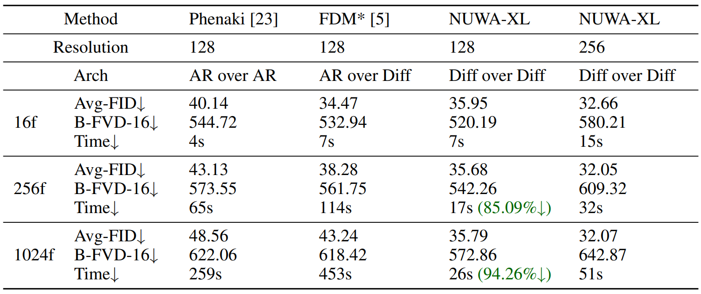
Comparison with the state-of-the-arts

The following is a quantitative comparison result of several state-of-the-art models.

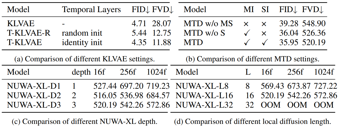
Ablation study

The following is the result of the ablation experiment.

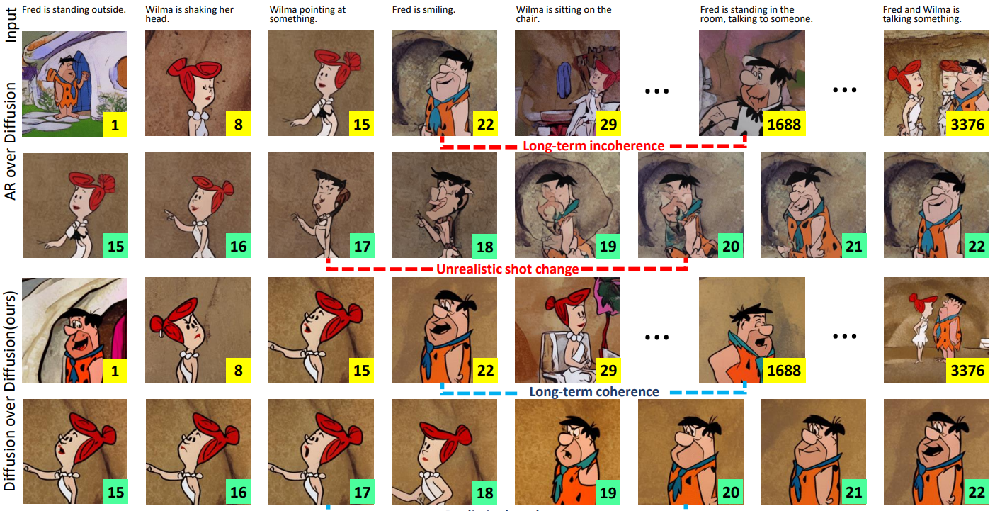
4. Qualitative results

The following is a qualitative comparison between AR over Diffusion and Diffusion over Diffusion.

Limitations

1. The effect of NUWA-XL was verified only for the publicly available cartoon Flintstones because long open domain videos (eg movies and TV programs) could not be used.
2. Direct training on long videos closes the gap between training and inference, but poses major challenges to the data.
3. NUWA-XL needs reasonable GPU resources for parallel inference to accelerate inference speed.