Blogs

NeurIPS 2022. [Paper] [Page] [Github]
Tim Brooks, Janne Hellsten, Miika Aittala, Ting-Chun Wang, Timo Aila, Jaakko Lehtinen, Ming-Yu Liu, Alexei A. Efros, Tero Karras
NVIDIA | UC Berkeley | Aalto University
7 Jun 2022

Introduction

Video is data that changes over time with complex patterns of camera viewpoint, motion, transformation, and occlusion. In some ways, video is off limits. Videos can last arbitrarily long and there is no limit to the amount of new content that can be displayed over time. But videos depicting the real world also need to be consistent with the laws of physics that dictate what changes are possible over time. For example, cameras can only move through 3D space along smooth paths, objects cannot transform into each other, and time cannot move backwards. Therefore, creating long, photorealistic videos requires the ability to generate endless new content while incorporating appropriate coherence.

In this paper, we focus on generating long videos with rich dynamics and new content occurring over time. Existing image generation models can produce ‘infinite’ images, but the type and amount of change along the time axis are very limited. For example, a synthetic infinite video of a person speaking contains only small movements of the mouth and head. Also, since typical video generation datasets often contain short clips with little new content over time, learning on short segments or frame pairs, forcing the content of a video to be fixed or having a small temporal receptive field You can bias your design choices to use your architecture.

The authors make the time axis the most important axis in video creation. To do this, we introduce two new datasets that include motion, changing camera viewpoints, and entry/exit points of objects and landscapes over time. The authors design a temporal latent representation that can learn long-term consistency and model complex temporal changes through learning on long videos.

The main contribution of this paper is a hierarchical generator architecture using a large temporal receptive field and novel temporal embeddings. It uses a multi-resolution strategy that first creates a low-resolution video and then refines it using a separate super-resolution network. We found that naive training on long videos at high spatial resolution is prohibitively expensive, but key aspects of the video persist at low spatial resolution. These observations allow us to learn from long videos in low resolution and short videos in high resolution, so we can prioritize the time axis and accurately depict long-term changes. Low-resolution and super-resolution networks are trained independently with an RGB bottleneck in between. This modular design allows each network to iterate independently and utilize the same super-resolution network for a variety of low-resolution networks.

Our method

There are two main challenges in modeling the long-term temporal behavior observed in real-world movies. First, a sufficiently long sequence must be used during training to capture the relevant effect. For example, using a pair of consecutive frames does not provide a meaningful learning signal for effects that occur over a few seconds. Second, the network itself must be able to operate over the long term. For example, if a generator’s receptive field spans only 8 adjacent frames, two frames that are more than 8 frames apart are not necessarily related to each other.

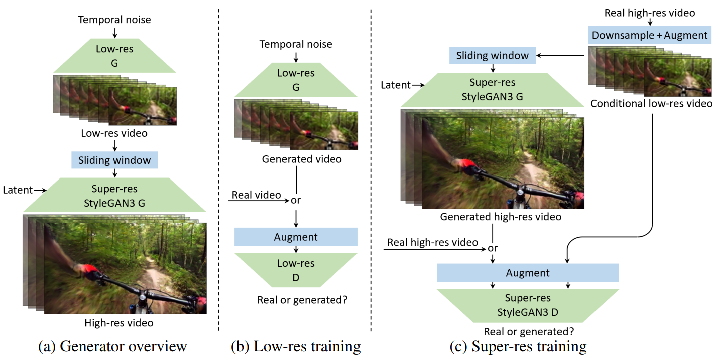
(a) in the figure above shows the overall design of the generator. We seed the generation process with a stream of variable-length temporal noise consisting of 8 scalar components per frame drawn from a Gaussian distribution. Temporal noise is first processed by a low-resolution generator to obtain a sequence of RGB frames with a resolution of $64^2, and then refined by a separate super-resolution network to produce a final frame with a resolution of $256^2. The role of the low-resolution generator is to model key aspects of motion and scene composition over time, which require strong expressive power and a wide receptive field, while the super-resolution network takes on the more granular task of generating the remaining details.

This two-level design offers maximum flexibility in terms of creating long movies. In particular, since the low-resolution generator is designed to be fully convolutional over time, the duration and time offset of the generated video can be controlled by shifting and reconstructing the temporal noise, respectively. On the other hand, super-resolution works on a frame-by-frame basis. It takes a short sequence of 9 consecutive low-resolution frames and outputs a single high-resolution frame. Each output frame is processed independently using a sliding window. The combination of fully-convolutional and per-frame processing allows for the generation of arbitrary frames in arbitrary order, which is highly desirable for interactive editing or real-time playback, for example.

Low-resolution and super-resolution networks are modular with an RGB bottleneck in between. This greatly simplifies experiments because the networks are trained independently and can be used in various combinations during inference.

1. Low-resolution generator

(b) in the figure above shows the learning settings for a low-resolution generator. At each iteration, we feed the generator a new temporary noise set, resulting in a sequence of 128 frames (4.3 seconds at 30 fps). To train the discriminator, a random video and a random interval of 128 frames within the video are selected and the corresponding sequence is sampled from the training data. The authors observed that training with long sequences tends to exacerbate the overfitting problem. As sequence length increases, it becomes more difficult for generators to simultaneously model temporal dynamics on multiple time scales, but at the same time discriminators find mistakes more easily. Indeed, the authors found that robust discriminator augmentation is required to stabilize learning. We use DiffAug with the same transform for each frame of the sequence and fractional time stretching between $\frac{1}{2} \times$ and $2 \times$.

Architecture

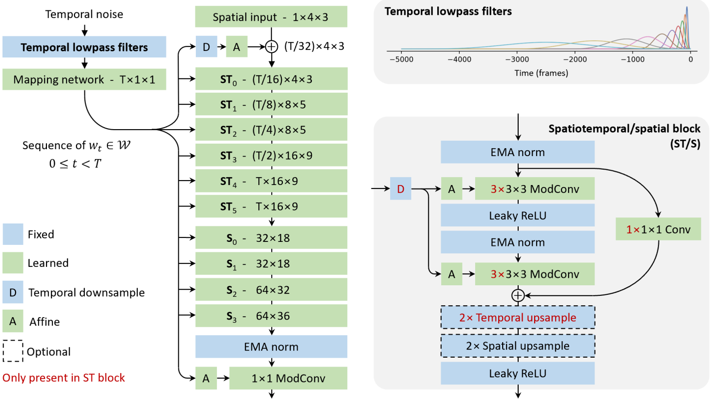
The figure above shows the architecture of a low-resolution generator. The main goal is to make the temporal axis the most important one, including careful design of temporal latent representation, temporal style modulation, space-time convolution and temporal upsample. This mechanism allows the generator to exhibit temporal correlations at multiple time scales across a vast temporal receptive field (5k frames).

We use a style-based design similar to StyleGAN3. We map the temporal noise input into a series of intermediate latents \(\{w_t\}\) that are used to modulate the motion of each layer in the main synthesis path. Each intermediate latent is associated with a specific frame, but through hierarchical 3D convolutions appearing in the base path, it can significantly affect the scene composition and temporal behavior of multiple frames.

To take full advantage of style-driven design, it is important to capture long-term temporal correlations, such as weather changes or persistent objects, at an intermediate latent. To do this, we first enrich the temporal noise input using a series of temporal lowpass filters and then pass it through a fully-connected mapping network on a frame-by-frame basis. The goal of lowpass filtering is to provide the mapping network with sufficient long-term context over various time scales. Specifically, given a stream of temporal noise $z(t) \in \mathbb{R}^8$, the corresponding rich expression $z’(t) \in \mathbb{R}^{128 \times 8}$ is calculated as $z_{i,j}’ = f_i \ast z_j$. Here, \(\{f_i\}\) is a set of 128 lowpass filters with a time range of 100 to 5000 frames, and $\ast$ represents a convolution with respect to time.

The main synthesis path starts by downsampling the time resolution of \(\{w_t\}\) to $32 \times$ and concatenating it with a constant learned at $4^2$ resolution. Then, focusing first on the temporal dimension (ST) and then on the spatial dimension (S), the temporal and spatial resolutions are gradually increased through a series of processing blocks shown in the lower right of the figure above. The first four blocks have 512 channels, then there are two blocks with 256, 128, and 64 channels, respectively. Processing block consists of the same basic building blocks as StyleGAN2 and StyleGAN3 with added skip connection. The intermediate activations are modulated according to copies of \(\{w_t\}\) that have been normalized and downsampled appropriately before each convolution. In practice, we use bilinear upsampling to remove boundary effects and use padding on the time axis. The combination of temporal latent representations and spatiotemporal processing blocks allows architectures to model complex and long-term patterns over time.

In the case of the discriminator, we use an architecture that prioritizes the temporal axis through a wide temporal receptive field, 3D space-time and 1D temporal convolutions, and spatial and temporal downsampling.

2. Super-resolution networks

The video super-resolution network is a simple extension of StyleGAN3 for conditional frame generation. Unlike low-resolution networks that output a series of frames and include explicit temporal operations, super-resolution generators output a single frame and use only temporal information from the input. Here, the actual low-resolution frame and 4 real low-resolution frames adjacent in time (a total of 9 frames) are concated along the channel dimension to provide context.

It removes the spatial Fourier feature input, resizes the low-resolution frame stack, and concats it to each layer throughout the generator. Generator architecture is unchanged from StyleGAN3, including the use of an intermediate latent code that is sampled per video. The low-resolution frames undergo augmentation prior to conditioning as part of the data pipeline to help ensure generalization over the generated low-resolution images.

The super-resolution discriminator is a simple extension of the StyleGAN discriminator, in which four low-resolution and high-resolution frames are concated to the input. The only other change was the removal of the minibatch standard deviation layer, which we decided was actually unnecessary. Low resolution and high resolution segments of 4 frames undergo adaptive augmentation where the same augmentation is applied to all frames of both resolutions. We also apply an aggressive dropout (p = 0.9 probability of zeroing the entire segment) to low-resolution segments so that the discriminator does not rely too heavily on the conditioning signal.

It’s surprising that such a simple video super-resolution model seems good enough to produce reasonably good high-resolution video. The authors focus mainly on low-resolution generators in their experiments and utilize a single super-resolution network trained per dataset. In the future, this simple network can be replaced with a more advanced model in a video super-resolution paper.

Datasets

Most existing video datasets introduce little or no new content over time. For example, a dataset of talking faces shows the same person for the duration of each video. UCF101 depicts a variety of human actions, but the video is short, camera movement is limited, and little or no new objects enter the video over time.

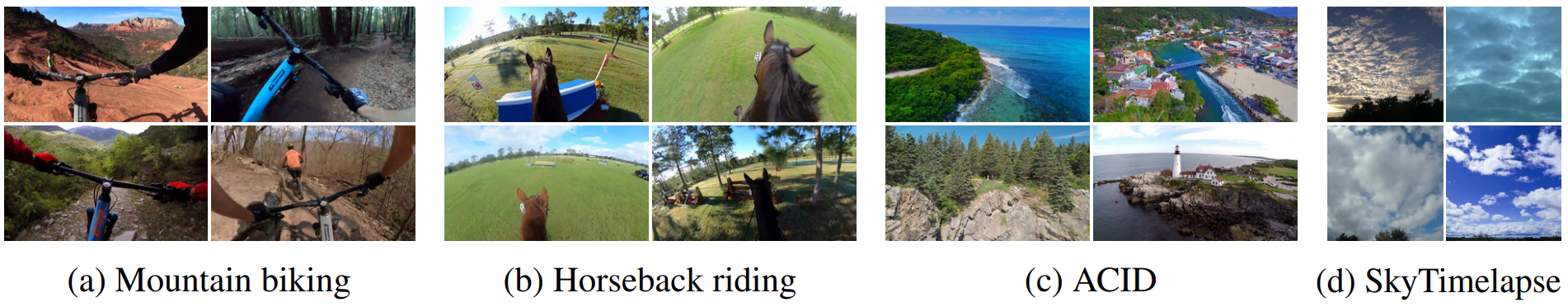
To best evaluate the model, we introduce two new video datasets, first-person mountain biking and horseback riding, which show complex changes over time. The new datasets in this paper include movement of a subject of a horse or cyclist, a first-person camera perspective moving through space, and new landscapes and objects over time. Videos are presented in high definition and have been manually trimmed to remove problematic areas, scene cuts, text overlays, and obstructed views. The mountain bike dataset contains 1202 videos with a median length of 330 frames at 30 fps, and the equestrian dataset contains 66 videos with a median length of 6504 frames at 30 fps.

We also evaluate the model on the ACID dataset, which contains significant camera motion but no other types of motion, and the commonly used SkyTimelapse dataset, which presents new content over time as clouds pass by, but the video is relatively homogeneous and the camera is kept fixed.

Results

1. Qualitative results

The following is an example of a qualitative result.

Videos created by various models can be found on the webpage.

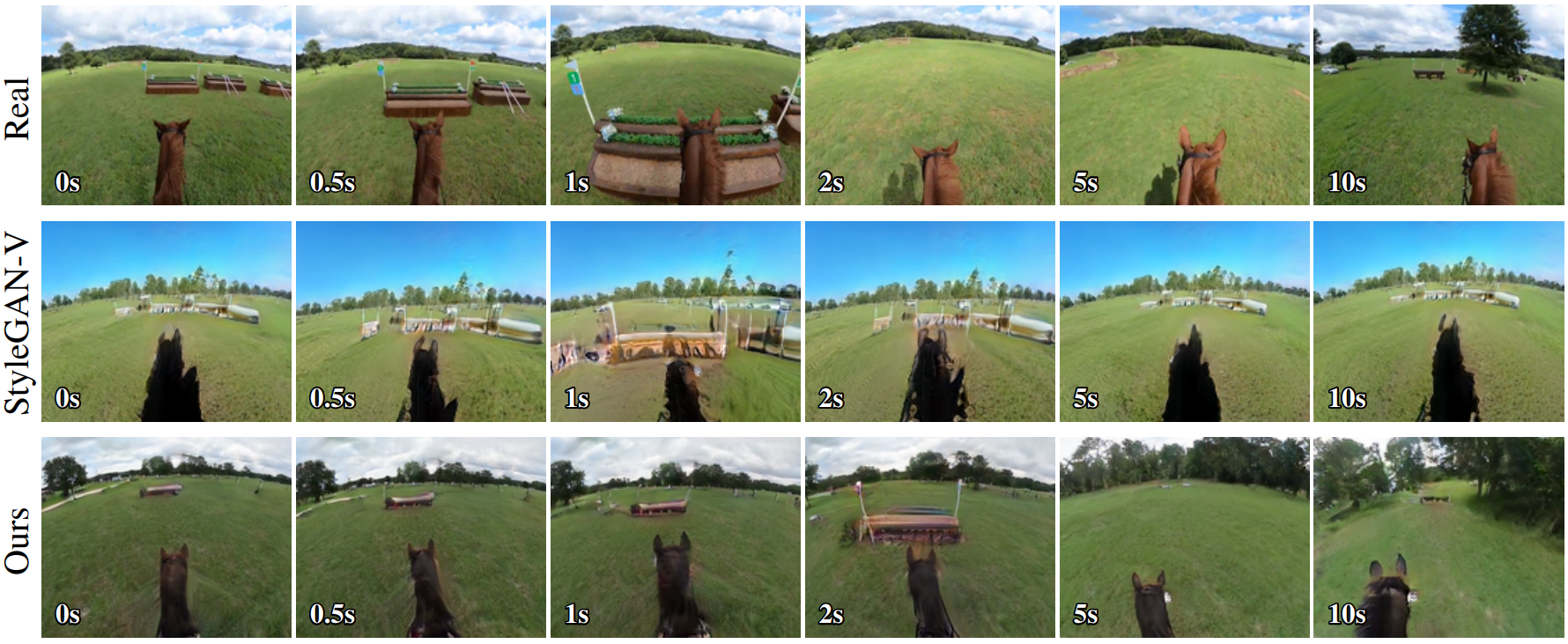
The main difference in the results is that our model generates realistically new content over time, whereas StyleGAN-V continuously repeats the same content. In the actual video, the scenery changes over time and the result emerges as the horse moves forward through space. However, the video generated by StyleGAN-V tends to transform back to the same scene at regular intervals. Similar repetitive content of StyleGAN-V is evident in all datasets. For example, the SkyTimelapse dataset shows that the clouds generated by StyleGAN-V move repeatedly back and forth. MoCoGAN-HD and TATS suffer from unrealistic rapid changes that diverge over time, and DIGAN results contain periodic patterns that can be seen both in space and time. The model in this paper can generate a continuous stream of new clouds.

2. Analyzing color change over time

The authors analyzed how the overall color scheme changes as a function of time to gain insight into how well it generates new content at a reasonable pace. Color similarity is measured by the intersection between the RGB color histograms. This serves as a simple proxy for real-world content changes and helps reveal biases in the model. $H(x, i)$ is the value of the histogram bin $i \in [1, \cdots, N^3]$ for the given image $x$ normalized such that $\sum_i H(x, i) = 1$ Represents a 3D color histogram function that computes values. Given a movie clip \(x = \{x_t\}\) and a frame interval $t$, we define color similarity as follows:

\[\begin{equation} S(x, t) = \sum_i \min (H(x_0, i), H(x_t, i)) \end{equation}\]

If $S(x, t)$ is 1, it means that the color histogram is the same for $x_0$ and $x_t$. In practice, the authors set $N = 20$ and measured the average and standard deviation of $S(\cdot, t)$ in 1000 random video clips containing 128 frames.

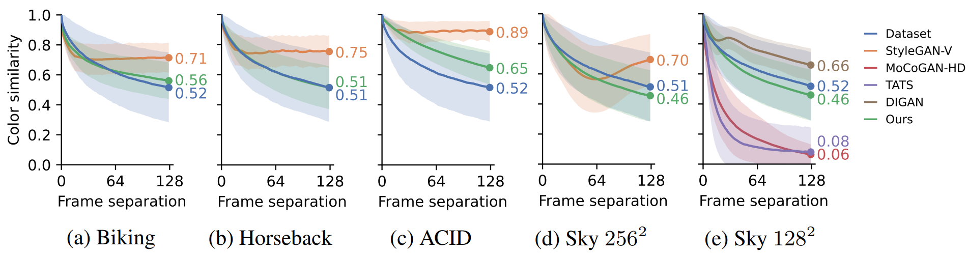
The figure above shows $S(\cdot, t)$ for real and generated videos in each dataset as a function of $t$. As the content and scenery gradually change, the curve slopes downward over time for real video. StyleGAN-V and DIGAN are biased toward changing colors too slowly. Both of these models include a fixed global latent code for the entire video. On the other hand, MoCoGAN-HD and TATS tend to change color too quickly. These models use RNNs and autoregressive networks, respectively, and both suffer from cumulative errors. The model in this paper almost matches the shape of the target curve and indicates that the color of the generated video changes at an appropriate speed.

3. Fréchet video distance (FVD)

The following table shows FVD calculations for segments of 128 frames and 16 frames.

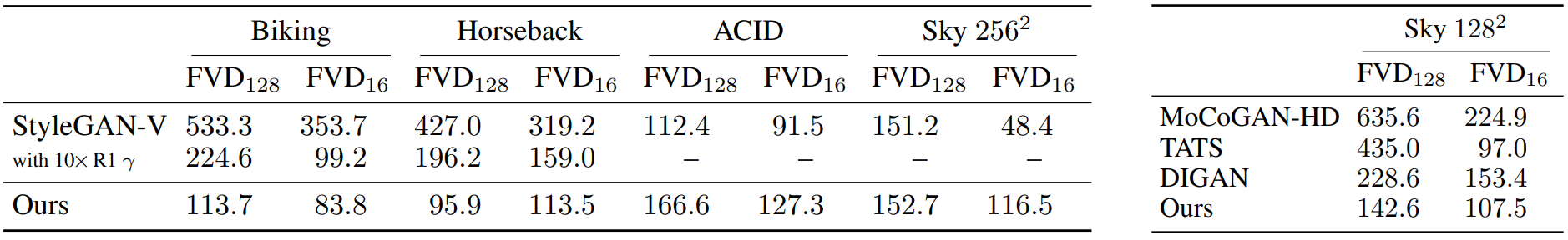
Looking at the left part of the table, our model outperforms StyleGAN-V on equestrian and mountain biking datasets containing more complex changes over time, but performs worse on ACID and in terms of $\textrm{FVD}_128$ SkyTimelapse performs slightly worse. However, this poor performance differs significantly from the conclusions of user studies. The authors attribute this discrepancy to the fact that StyleGAN-V produces better individual frames and probably better small-scale motion, but is severely lacking in reproducing reliable long-term realism, and FVD is primarily sensitive to electronic aspects. .

The right side of the table is the FVD measurement for SkyTimelapse at $128^2$. In this comparison, our model outperforms all baslines in terms of $\textrm{FVD}_128$.

4. Ablations

The following is a table showing the ablation results for the learning sequence length and the temporal lowpass filter footprint.

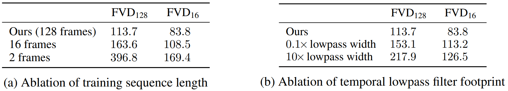
Looking at (a), we can see that watching long videos during training helps the model learn long-term consistency. (b) shows the negative impact of using improperly sized filters.

The following shows the effect of a super-resolution network.

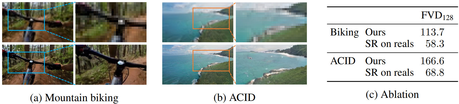
(a) and (b) show examples of low-resolution frames generated from the model along with corresponding high-resolution frames generated from the super-resolution network. It can be confirmed that super-resolution networks generally perform well. To ensure that the quality of the results is not disproportionately limited by the super-resolution network, we additionally measure the FVD when feeding the actual low-resolution video to the super-resolution network as input. Looking at (c), the FVD is actually greatly improved in this case, indicating that there are significant gains to be realized by further improving the low-resolution generator.