


SIGGRAPH Asia 2021. [Paper] [Page] [Github]
Yuanxun Lu, Jinxiang Chai, Xun Cao
Nanjing University | Xmov
22 Sep 2021

Introduction
Talking-head animation, ie compositing video frames that are in sync with the target’s audio, is useful for interactive applications. Recent advances in deep learning have made great strides in this age-old problem. However, realizing realistic and expressive talking animations is still a challenge. Humans are extremely sensitive to facial artifacts, which places high demands on the desired technology.
Several factors contribute to the difficulty of creating talking-head animations.
- In addition to the difficulty of mapping from a one-dimensional audio signal to a facial movement placed on a high-dimensional manifold, there is a difficulty in failing to preserve the speech characteristics of each due to the domain difference between the audio and the target voice space.
- Head and body movements are not closely related to audio. For example, they may shake their head or stay still when saying the same word, which depends on many factors such as mood, location or past poses.
- Compositing controllable photorealistic renderings is not trivial. Traditional rendering engines are still far from what you want, and the result can be perceived as fake at a glance. Neural renderers wield great power for photorealistic rendering, but performance degradation occurs when the predicted motion is far outside the bounds of the training corpus.
- In many interactive scenarios, such as video conferencing or digital avatars, the entire system needs to run in real-time, which demands a lot of system efficiency without compromising performance.
In this paper, we propose a deep learning architecture called Live Speech Portraits (LSP) to solve these problems and take a step forward towards practical applications. The system in this paper generates personalized talking-head animation streams, including audio-driven facial expressions and motion dynamics (head posture and upper body motion), and realistically renders them in real time.
First of all, the authors adopt the idea of self-supervised representation learning, which shows great power in learning semantic or structural representations and helps in various downstream tasks to extract speaker-independent audio features. To create realistic and personalized animations from audio streams, audio features are further projected into the target feature space and reconstructed using the target features. This process can be viewed as domain adaptation from source to target. After that, the mapping from the reconstructed audio features to facial dynamics can be learned.
Another important component contributing to realistic talking-head animation is head and body movement. To generate a personalized and time-coherent head pose from audio, we assume that the current head pose is partly related to audio information and partly related to previous poses. Based on these two conditions, the authors propose a new autoregressive probabilistic model for learning the target’s head pose distribution. Head poses are sampled from the estimated distribution, and upper body movements are additionally inferenced from the sampled head poses.
To synthesize photorealistic renderings, we use image-to-image transformation networks conditioned on feature maps and candidate images. A landmark image is created as an intermediate representation by applying the sampled head pose to the facial dynamics and projecting the transformed facial keypoints and upper body positions onto the image plane. Although the system in this paper consists of several modules, it is small enough to run in real time at over 30 fps.
Method
Given an arbitrary audio stream, the Live Speech Portraits (LSP) approach creates realistic talking-head animations of the target in real time. The approach in this paper consists of three steps: deep speech expression extraction, audio-to-face prediction, and realistic face rendering.
The first step extracts the speech representation of the input audio. Representation extractors learn high-level speech representations and are trained in a self-supervised manner on an unlabeled speech corpus. We then project the representation into the speech space of the target to improve generalization. The second step predicts the overall motion dynamics. Two elaborately designed neural networks predict mouth-related motions and head poses in speech expressions, respectively. Mouth-related motions are represented by sparse 3D landmarks and head poses by fixed rotations and translations. Considering that head poses have less to do with audio information than mouth-related motions, we use a stochastic autoregressive model to learn poses conditional on audio information and previous poses. Other facial features that have little correlation with the audio (eg eyes, eyebrows, nose, etc.) are sampled from the training set. Then compute upper body motion from the predicted head pose. In the final step, we use a conditional image-to-image transformation network to synthesize realistic video frames from the previous predictions and candidate image sets.
1. Deep Speech Representation Extraction
The input information, the voice signal, plays an important role because it supplies power to the entire system. We learned high-level speaker-independent speech representations from surface features by utilizing a deep learning approach that is typically learned from self-supervised mechanisms.
Specifically, we use an autoregressive predictive coding (APC) model to extract structured speech representations. APC models predict future surface features given prior information. We choose the 80-dimensional log Mel spectrogram as the voice surface feature. The model is a standard 3-layer unidirectional gated recurrent unit (GRU).
\[\begin{equation} h_l = \textrm{GRU}^{(l)} (h_{l-1}), \quad \forall l \in [1, L] \end{equation}\]Here, $h_l \in \mathbb{R}^{512}$ is the hidden state of each layer of GRU. The hidden state of the last GRU layer is used as a deep voice representation. The output is mapped by adding a linear layer to predict the future logMel spectrogram during training, and this linear layer is removed after training.
Manifold Projection
People possess different speaking styles that are considered personalized styles. Direct application of deep speech representations can lead to erroneous results when the input speech representation is located far away from the speech feature space of the target. To improve generalization, manifold projection is performed after extracting speech expressions.
The manifold projection operation is inspired by the recent success of compositing faces from sketches, which can be generalized to sketches far from human faces. We apply the locally linear embedding (LLE) assumption to the speech representation manifold. Each data point and its neighbors are LLEs in the high-dimensional manifold.
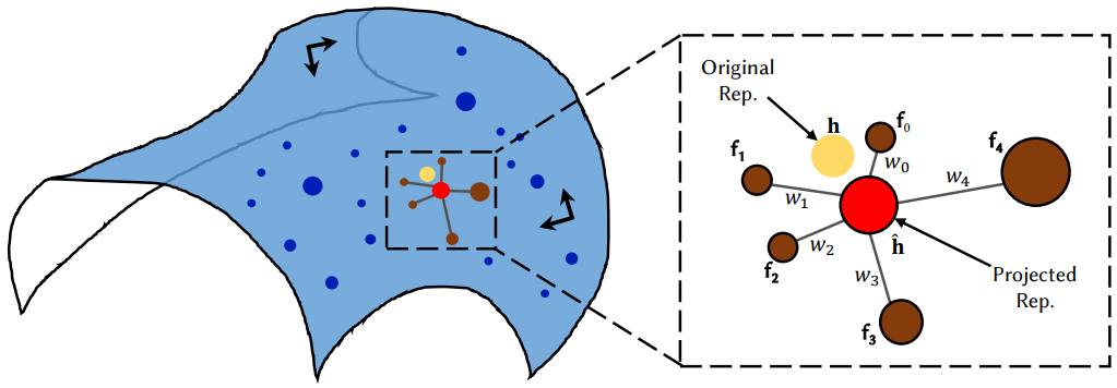
Given an extracted speech expression $h \in \mathbb{R}^{512}$, the reconstructed expression $\hat{h} \in \mathbb{R}^{512}$ under the LLE assumption for each dimension Calculate. As depicted in the figure above, first calculate the Euclidean distance of $K$ points close to $h$ in the target speech expression database $\mathcal{D} \in \mathbb{R}^{N_s \times 512}$ to find $N_s$ is the number of learning frames. Then find the linear combination of $K$ points that best reconstruct $h$. This is equivalent to calculating the coordinates of the center of $h$ based on its neighbors by solving the following minimization problem.
where $w_k$ is the centroid weight of $k$-nearest neighbor $f_k$ and can be calculated by solving the least squares problem. $K$ was empirically chosen to be 10 in the experiment. Finally, we get the projected speech expression $\hat{h}$.
\[\begin{equation} \hat{h} = \sum_{k=1}^K w_k \cdot f_k \end{equation}\]Then, $h$ is sent to the motion predictor as the input deep speech representation.
2. Audio to Mouth-related Motion
Predicting mouth-related movements from audio has been extensively studied over the past few years. People use deep learning architectures to learn mappings from audio features to intermediate representations, such as lip-related landmarks, parameters of a parametric model, 3D vertices, or face blend shapes. In this paper, the 3D displacement $\Delta v_m \in \mathbb{R}^{25 \times 3}$ for the average position of the target in object coordinates is used as an intermediate expression.
To model the sequence dependencies, we use an LSTM model to learn the mapping from voice representations to mouth-related actions. Adds a $d$ frame delay to make the model accessible in the short future, greatly improving quality. Afterwards, the output of the LSTM network is fed to the MLP, and finally the 3D displacement $\Delta v_m$ is predicted. In summary, the mouth-related prediction module works as follows.
\[\begin{equation} m_0, m_1, \cdots, m_t = \textrm{LSTM} (\hat{h}_0, \hat{h}_1, \cdots, \hat{h}_{t+d}), \quad \Delta v_{m, t} = \textrm{MLP} (m_t) \end{equation}\]Here, the time delay $d$ is set to 18 frames equal to 300 ms delay (60 FPS) in the experiment. LSTM is stacked with three layers, each layer has a hidden state of size 256. The MLP decoder network has three layers with hidden state sizes of 256, 512, and 75.
3. Probabilistic Head and Upper Body Motion Synthesis
Head pose and upper body movement are two other components that contribute to vivid talking-head animation. For example, when people speak, they naturally shake their heads and move their bodies to express their emotions and convey their attitudes to their audience.
Head pose estimation in audio is important because there are few relationships between them. Given the inherent difficulty of one-to-many mapping from audio to head poses, we make two assumptions as prior knowledge.
- Head pose is in part related to audio information such as expression and intonation. For example, people tend to nod when expressing agreement and nod when speaking with a high accent, and vice versa.
- The current head pose is partially dependent on the past head pose. For example, people are more likely to turn their heads if you’ve turned them at a big angle before.
These two assumptions simplify the problem and motivate the architecture design. The proposed network $\phi$ should have the ability to see conditionally the previous head pose and the current audio information. Furthermore, instead of treating it as a regression problem and learning it using the Euclidean distance loss, we should model this mapping as a probability distribution. Recently, probabilistic models are successfully used for motion synthesis and outperform deterministic models. The joint probability of head motion can be expressed as:
\[\begin{equation} p(x \vert \hat{h}) = \prod_{t=1}^T p(x_t \vert x_1, x_2, \cdots, x_{t-1}, \hat{h}_t) \end{equation}\]where $x$ is the head movement and $\hat{h}$ is the speech expression.
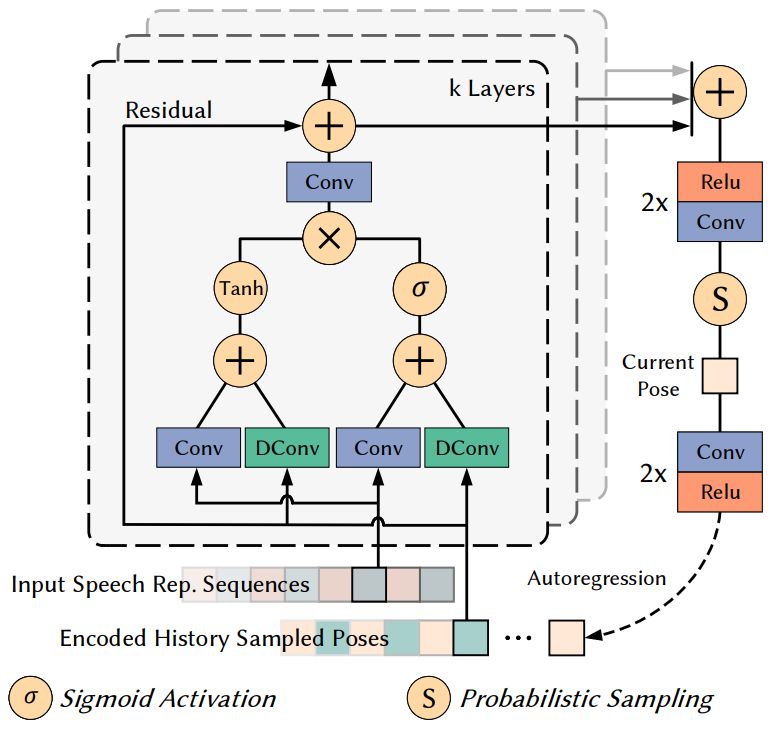
The probability model used in this paper is a multidimensional Gaussian distribution. The network architecture is inspired by the recent success of conditional stochastic generative modeling. The detailed design of the probabilistic model is illustrated in Figure 4 above.
The model is a stack of two residual blocks with 7 layers each. Considering the long-time dependencies required to generate natural head movements (a single shake of the head from left to right can last for several seconds), these residual blocks use a dilation convolution layer instead of a normal convolution with much fewer parameters to determine the dependencies. capture The dilation is doubled 7 times for each layer of the architecture and then repeated twice: 1, 2, 4, 8, 16, 32, 64, 1, 2, 4, 8, 16, 32, 64. As a result, the model The receptive field size $F$ for the previous head pose of is 255 frames, corresponding to 4.25 seconds in the experiment. The output of each layer is summed and processed by a post-processing network (a stack of two relu-conv layers) to produce the current distribution.
In particular, the model outputs the mean $\mu$ and standard deviation $\sigma$ of the estimated Gaussian. Then sample from the distribution to get a final head pose $P \in \mathbb{R}^6 consisting of 3D rotation $R \in \mathbb{R}^3$ and transition $T \in \mathbb{R}^3$ get $ The authors also tried with a Gaussian mixture model, but found no significant improvement. After sampling, the current pose is encoded as input pose information for the next timstep to form an autoregressive mechanism. In summary, head pose estimation can be expressed as:
\[\begin{equation} P_{para, t} = \phi (P_{t-F}, \cdots, P_{t-1}, \hat{h}_t) \\ P_t = \textrm{Sample} (P_{para, t}) \end{equation}\]Upper Body Motion
An ideal method for upper body motion estimation is to build a body model and estimate its parameters. To avoid overcomplicating the algorithm, we assign the torso as a billboard shaped with several manually defined shoulder landmarks. The initial depth of the Billboard is set to the average depth of the landmarks over the entire training sequence and is the same for all. In most cases, we use the resulting billboard model with 50% of the transition part $T$ in the predicted head motion $P$.
4. Photorealistic Image Synthesis
The last step is to generate realistic face renderings from previous predictions. The rendering network is inspired by recent advances in photorealistic and controllable face animation synthesis. We use a conditional image-to-image transformation network with adversarial learning as the backbone. The network creates a photorealistic rendering by channel-wise concating the conditional feature map and the target’s candidate images $N = 4$.
Conditional Feature Maps
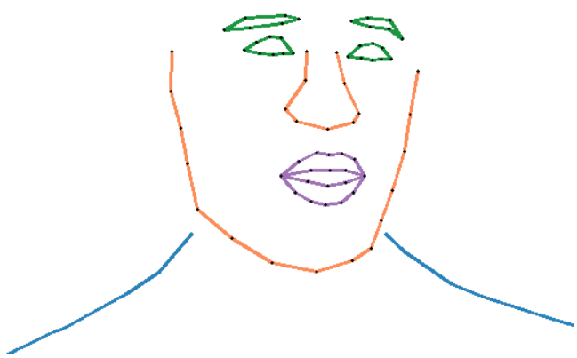
Draw conditional feature maps for each frame in the above prediction to provide face and upper body cues. An example of a conditional map is shown in the figure above. The feature map consists of a face part and an upper body part. If you draw a semantic area or even a single area with color, one channel takes more information and more drawing time. The authors did not find any significant improvement in these two alternatives. Faint face landmarks and the expected upper body billboard can be found in object coordinates. Therefore, these 3D positions must be projected onto a 2D image plane through the pre-calculated camera-specific parameters $K$. The camera model used is a pinhole camera model.
Here $f$ is the focal length and $f(c_x, c_y)$ is the principle point. Consecutive 2D projection components are concatenated in a predefined semantic order to create conditional feature maps of size $1 \times 512 \times 512$.
Candidate Image set
In addition to the conditional feature map, a set of candidate images of the target person is additionally input to provide detailed scene and texture clues. The authors found that adding these candidate sets helps the network generate a consistent background by taking into account the changing camera movements in the training set, relieving the network’s pressure to synthesize subtle details such as teeth and pores.
These images are automatically selected. Select the 100th min/max mouth region for the first two. The rest samples the x- and y-axis rotations at regular intervals and picks the closest sample in the interval. Therefore, the size of the final concated input image is $13(1+3 \times 4) \times 512 \times 512$.
The network is an 8-layer UNet-like CNN with skip connections at each resolution layer. The resolution of each layer is ($256^2$, $128^2$, $64^2$, $32^2$, $16^2$, $8^2$, $4^2$, $2^2$), and each channel The number is (64, 128, 256, 512, 512, 512, 512, 512). Each encoder layer consists of one convolution (stride 2) and one residual block. The symmetrical decoder layer is almost identical except that the first convolution is replaced by a nearest upsampling operation with a scale factor of 2.
Implementation Details
1. Dataset Acquisition and Pre-processing
We apply the approach of this paper to 8 target sequences of 7 subjects for learning and testing. These sequences span the 3-5 minute range. All videos are extracted at 60FPS and synchronized audio waves are sampled at 16Khz frequency.
First crop the video to keep the face centered, then resize it to 512 $\times$ 512. All input and output images share the same resolution. Divide the video into 80% / 20% for training and evaluation.
Detect 73 predefined facial landmarks for every video using a commercial tool. It uses an optimization-based 3D face tracking algorithm to provide ground-truth of 3D mouth shape and head pose. For camera calibration, a binary search is used to calculate the focal length f. Set the origin (c_x, c_y) to the center of the image. It performs camera calibration and 3D face tracking on the original image, and computes a transformation matrix according to cropping and resizing parameters. The feature points of the upper body movements are manually selected once for the first frame of each sequence and tracked for the remaining frames using LK optical flow and OpenCV implementation.
To train the APC speech expression extractor, we use the Chinese portion of the Common Voice dataset that provides unlabeled utterances. Specifically, the subset contained 889 different speakers with various accents. There are a total of about 26 hours of unlabeled utterances.
An 80-dimensional log Mel spectrogram is used as the surface feature. The Log Mel spectrogram is calculated with a 1/60 second frame length, 1/120 second frame shift, and a 512-point Short-Time Fourier Transform (STFT). The APC model was trained in Mandarin Chinese, but the system still works well in other languages as the model learns high-level semantic information. Manifold projection also improves generalization ability.
2. Loss Functions
Deep Speech Representation Extraction
The training of the APC model is fully self-supervised through surface feature prediction before $n$ frames. Given a sequence of log Mel spectrograms $(x_1, x_2, \cdots, x_T)$, the APC model processes each element $x_t$ in timestep $t$ and predicts Output $y_t$ to generate the prediction sequence $(y_1, y_2, \cdots, y_T)$. Optimize the model by minimizing the L1 loss between the input sequence and prediction as follows.
\[\begin{equation} \sum_{i=1}^{T-n} | x_{i+n} - y_i | \end{equation}\]Here we set $n = 3$.
Audio to Mouth-related Motion
To learn the mapping from audio to mouth-related motion, we minimize the $L_2$ distance between the actual mouth displacement and the predicted displacement. In particular, the loss can be written as
\[\begin{equation} \sum_{t=1}^T \sum_{i=1}^N \| \Delta v_{m,t} - \Delta \hat{v}_{m,t} \|_2^2 \end{equation}\]Here, $T = 240$ represents the number of consecutive frames sent to the model in each iteration. $N = 25$ is the predefined number of mouth-related 3D points in the experiment.
Probabilistic Head Motion Synthesis
In addition to learning the mapping from audio to mouth-related motions, we aim to estimate the target’s head pose during training. Upper body motion can be inferred from the head pose. In particular, we use an autoregressive model to model the head pose distribution. We train the model by minimizing the negative log-likelihood of the pose distribution. Given a sequence of previous head poses $(x_{t-F}, \cdots, x_t)$ and speech expressions $h_t$, the stochastic loss is
\[\begin{equation} -\log (\mathcal{N} (x_t, h_t \vert \hat{\mu}_n, \hat{\sigma}_n)) \end{equation}\]This loss term forces the model to output the mean $\hat{\mu}_n$ and $\hat{\sigma}_n$ of the Gaussian distribution. To increase numerical stability, output $-\log (\hat{\sigma}_n)$ instead of $\hat{\sigma}_n$. Each element of the pose sequence $x_t \in \mathbb{R}^12$ is the current pose $p_t \in \mathbb{R}^6$ and the linear velocity term $\Delta p_t \in \mathbb{R}^6$ consists of After sampling from the distribution, we only use rotations and transitions in the first six dimensions, but adding these velocity terms implicitly forces the model to focus on the velocity of the motion, resulting in smoother results.
Photorealistic Image Synthesis
Finally, a neural renderer is trained to synthesize a realistic talking person image. The learning process follows an adversarial learning mechanism. Multi-scale PatchGAN architecture is adopted as the backbone of discriminator $D$. The image-to-image transformation network $G$ is trained to generate realistic images to fool the discriminator $D$, while the discriminator $D$ is trained to say that it is a generated image. In particular, we optimize the discriminator $D$ using the LSGAN loss as the adversarial loss.
\[\begin{equation} \mathcal{L}_{GAN} (D) = (\hat{r} - 1)^2 + r^2 \end{equation}\]Here, $\hat{r}$ and $r$ are the classification output of the discriminator when inputting the ground-truth image $\hat{y}$ and the generated rendering $y$, respectively. The authors additionally used color loss \(\mathcal{L}_C\), perceptual loss \(\mathcal{L}_P\), and feature matching loss \(\mathcal{L}_{FM}\).
\[\begin{equation} \mathcal{L}_G = \mathcal{L}_{GAN} + \lambda_C \mathcal{L}_C + \lambda_P \mathcal{L}_P + \lambda_{FM} \mathcal{L}_{FM} \ \ \mathcal{L}_{GAN} = (r - 1)^2 \end{equation}\]The weights $\lambda_C$, $\lambda_P$, and $\lambda_{FM}$ were set to 100, 10, and 1, respectively. The color loss is the $L_1$ per-pixel loss of the generated image $y$ and the ground-truth image $\hat{y}$.
\[\begin{equation} \mathcal{L}_C = \| y - \hat{y} \|_1 \end{equation}\]It is said that if the weight is applied to the mouth 10 times larger, the error related to the mouth decreases, but the error of the entire image increases.
For perceptual loss, we use the VGG19 network to extract perceptual features from $\hat{y}$ and $y$ and minimize the $L_1$ distance between features.
\[\begin{equation} \mathcal{L}_P = \sum_{i \in S} \| \phi^{(i)} (y) - \phi^{(i)} (\hat{y}) \|_1 \end{equation}\]Here, \(S = \{1, 6, 11, 20, 29\}\) represents the layer used.
Finally, feature matching loss is used to improve learning speed and stability.
\[\begin{equation} \mathcal{L}_{FM} = \sum_{i=1}^L \|r - \hat{r} \|_1 \end{equation}\]where $L$ is the number of spatial layers of the discriminator $D$.
3. Training Setup and Parameters
- Adam optimizer ($\beta_1 = 0.9$, $\beta_2 = 0.999$)
- Learning rate = $10^{-4}$, decreasing linearly to $10^{-5}$
- Using Nvidia 1080Ti GPU
4. Real-Time Animation
It takes a total of 27.4 ms to inference for more than 30 FPS on Intel Core i7-9700K CPU (32 GB RAM) and NVIDIA GeForce RTX 2080 (8 GB RAM).
Results
1. Qualitative Evaluation
The following is the result of audio-based talking-head animation.

The following shows the pose control possibility of the method of this paper.

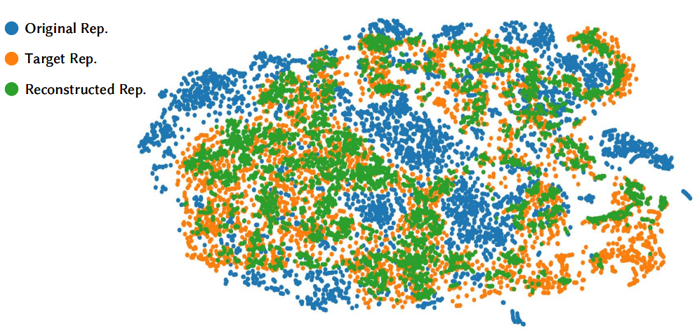
Here is a t-SNE visualization of the manifold projection.
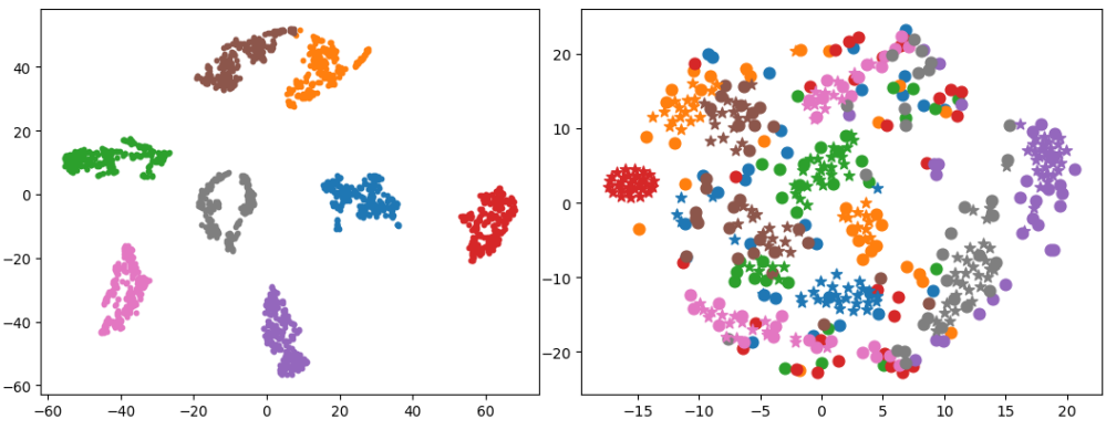
Here is a t-SNE visualization of head pose generation. The left side is a visualization of the generated pose, and the right side is a visualization of the generated pose (★) and the head pose (●) of the training corpus.
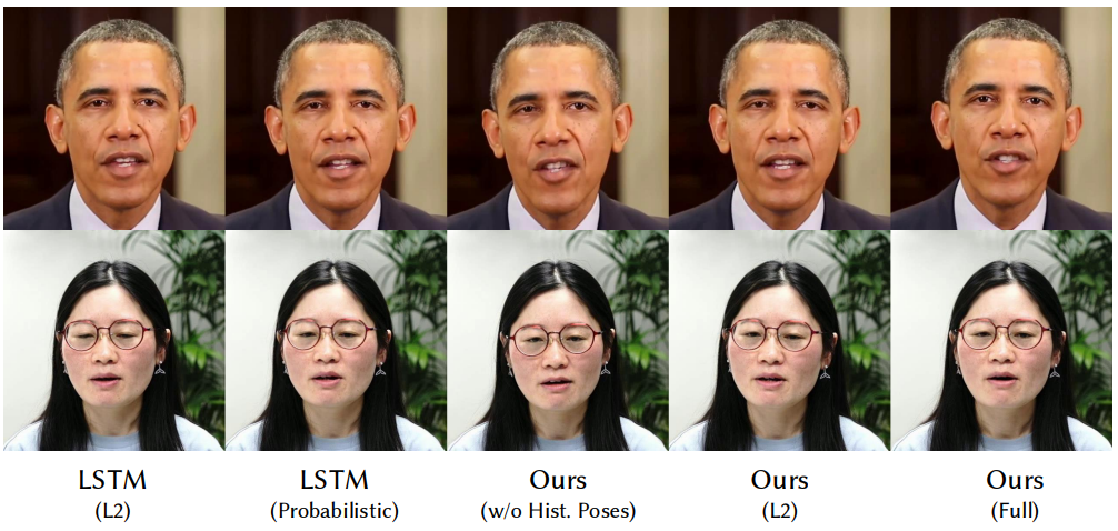
The following is a qualitative comparison of the estimated head poses.
2. Quantitative Evaluation
The following is the measurement of the Euclidean distance between landmarks according to the time delay $d$.

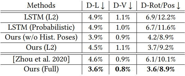
The following is a quantitative evaluation result for head pose prediction.
The following is the result of qualitative evaluation of the renderer’s conditional input.

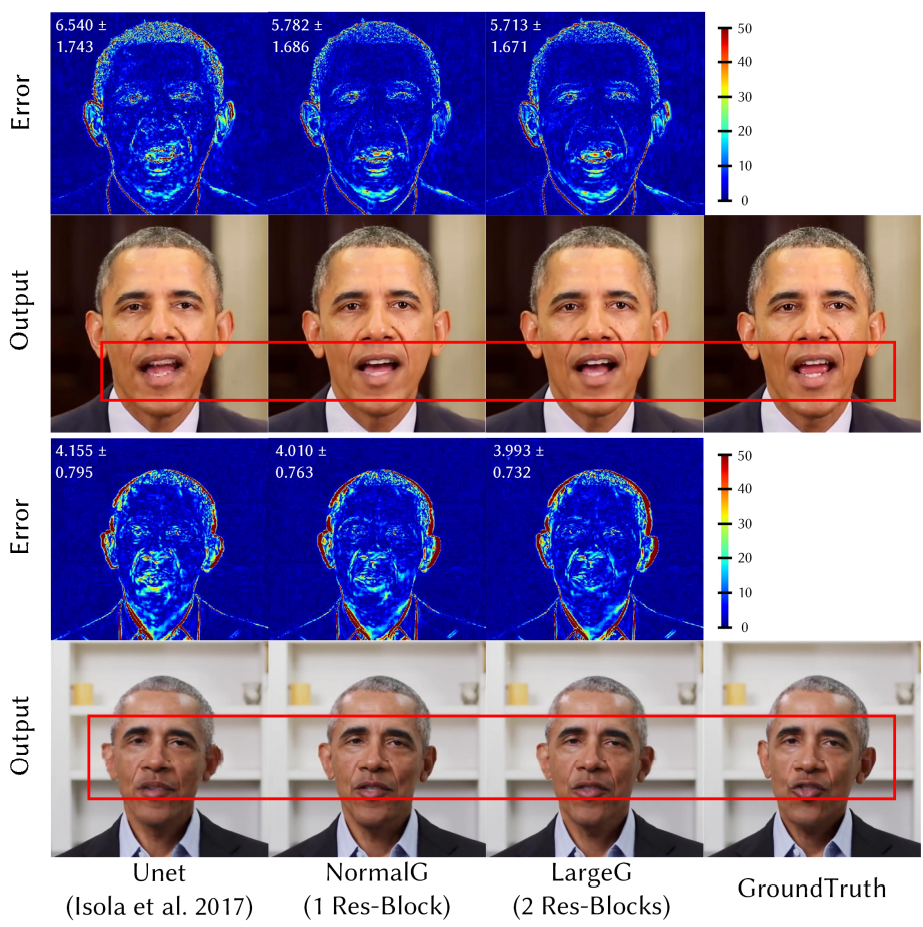
The following is the qualitative evaluation result of the renderer’s architectural design.
The following is a qualitative evaluation result on the size of the training dataset.

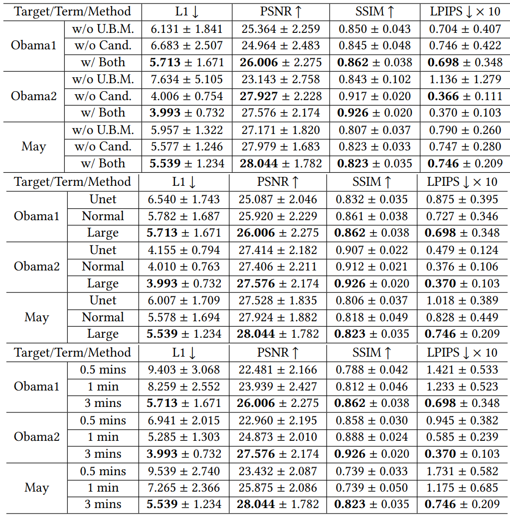
The following are quantitative evaluation results for conditional input (top), architecture (middle), and training dataset size (bottom).
3. Comparisons to the State-of-the-Art
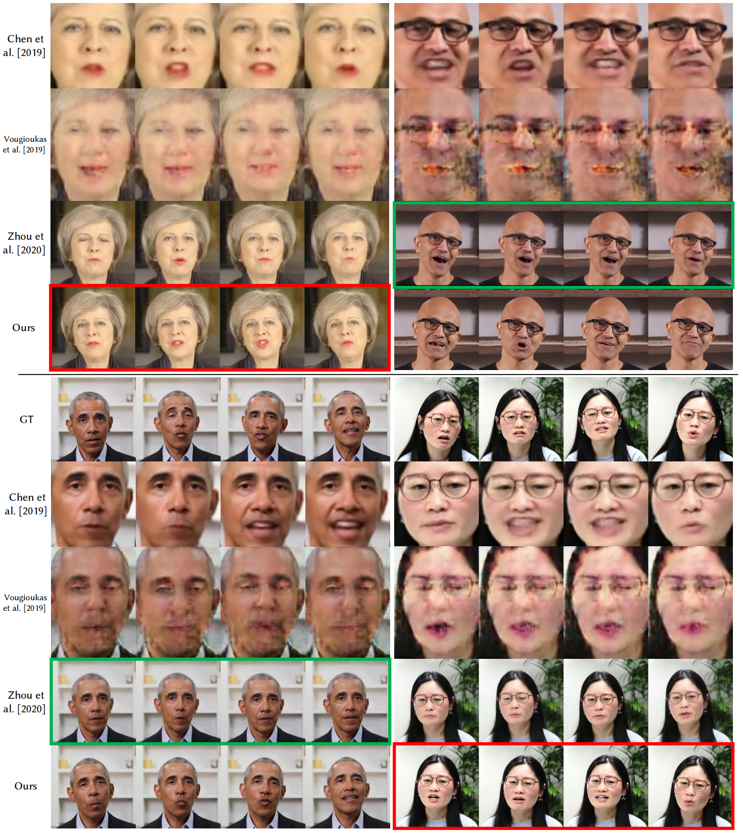
Here’s a comparison with the state-of-the-art image-based generation method.
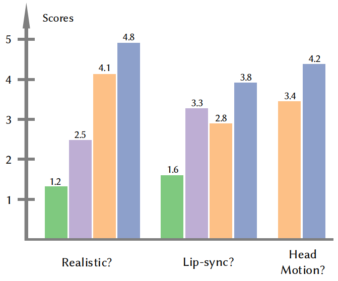
4. User Study
The following are the results of three user studies.
![[Paper review] Self-correcting LLM-controlled Diffusion Models](/assets/images/blog/post-5.jpg)