[Paper review] HyperStyle: StyleGAN Inversion with HyperNetworks for Real Image Editing

CVPR 2022. [Paper] [Page] [Github]
Yuval Alaluf, Omer Tov, Ron Mokady, Rinon Gal, Amit H. Bermano
Blavatnik School of Computer Science, Tel Aviv University
30 Nov 2021

Introduction

GANs, especially StyleGANs, have become the standard for image synthesis. Thanks to semantically rich latent representations, many tasks facilitate diverse and expressive editing through latent space manipulation. However, a major challenge in adopting this approach for real-world applications is the ability to edit real-world images. To edit a real photo, you first need to find its latent representation through a process commonly referred to as GAN inversion. The inversion process is a well-studied problem, but it is still an open challenge.

Recent studies have shown the trade-off between distortion and editability. You can invert the image into the well-behaved region of StyleGAN’s latent space and get good editing possibilities. However, these regions are generally less expressive and thus less faithfully reconstructed into the original image. Recently, Pivotal Tuning Inversion (PTI) showed that this trade-off can be avoided by considering a different approach to inversion. Instead of searching for the latent code that most accurately reconstructs the input image, we fine-tune the generator to insert target IDs into well-behaved regions of the latent space. In doing so, it demonstrated state-of-the-art reconstruction while maintaining a high level of editability. However, this approach relies on image-by-image optimization of the generator, which is expensive and takes up to 1 minute per image.

A similar time-accuracy trade-off can be observed in the classic inversion approach. At one end of the spectrum, latent vector optimization approaches achieve impressive reconstructions, but are impractical at scale, taking minutes per image. On the other hand, encoder-based approaches leverage rich datasets to learn mappings from images to latent representations. These approaches work in fractions of a second, but are generally less faithful to reconstruction.

In this paper, we aim to apply PTI’s generator tuning technology to an encoder-based approach and bring it to the realm of interactive applications. It does this by introducing a hypernetwork that learns how to subdivide the generator weights for a given input image. The hypernetwork consists of a lightweight feature extractor (ex. ResNet) and a set of refinement blocks for each StyleGAN convolution layer. Each refinement block is responsible for predicting offsets for the convolution filter weights of that layer.

A major challenge in designing such a network is the number of parameters constituting each convolution block that needs to be refined. Simple prediction of the offset for each parameter requires a hypernetwork with more than 3 billion parameters. We explore several ways to reduce this complexity.

Offset sharing between parameters
Share network weights between different hypernetwork layers
An approach inspired by depth-wise convolution

Finally, we observe that the reconstruction can be further improved through an iterative refinement method that gradually predicts the desired offset through a small number of forward passes through the hypernetwork. In doing so, HyperStyle, the approach of this paper, learns how to optimize generators in an inherently efficient way.

The relationship between HyperStyle and existing generator tuning methods can be seen as similar to that between encoders and optimization inversion methods. Just as an encoder finds a desired latent code through a trained network, a hypernetwork efficiently finds a desired generator without image-specific optimization.

Method

1. Preliminaries

In solving the GAN inversion task, the goal of this paper is to identify a latent code that minimizes the reconstruction distortion for a given target image $x$.

\[\begin{equation} \hat{w} = \underset{w}{\arg \min} \mathcal{L} (x, G(w; \theta)) \end{equation}\]

Here, $G(w; \theta)$ is an image generated as latent $w$ by pretrained generator $G$. $\mathcal{L}$ is the loss, usually $L_2$ or LPIPS is used. Solving the equation above with optimization typically takes several minutes per image. To reduce the inference time, the encoder $E$ is applied to the large image set $\{x^i\}_{i=1}^N$.

\[\begin{equation} \sum_{i=1}^N \mathcal{L} (x^i, G (E (x^i); \theta)) \end{equation}\]

can be trained to minimize This creates a fast inference procedure $\hat{w} = E(x)$. Latent manipulation $f$ can be applied to the inverted code $\hat{w}$ to get the edited image $G(f(\hat{w}); \theta)$.

Recently, PTI proposed injecting new IDs into well-behaved regions of StyleGAN’s latent space. Given a target image, an optimization process is used to find the initial latent $\hat{w}_{init} \in \mathcal{W}$ leading to the approximate reconstruction. This is followed by fine-tuning where the generator weights are adjusted so that the same latent better reconstructs a particular image.

\[\begin{equation} \hat{\theta} = \underset{\theta}{\arg \min} \mathcal{L}(x, G(\hat{w}_{init}; \theta)) \end{equation}\]

Here $\hat{\theta}$ represents the new generator weight. The final reconstruction can be obtained as $\hat{y} = G(\hat{w}_{init}; \hat{\theta})$ using the initial inversion and modified weights.

2. Overview

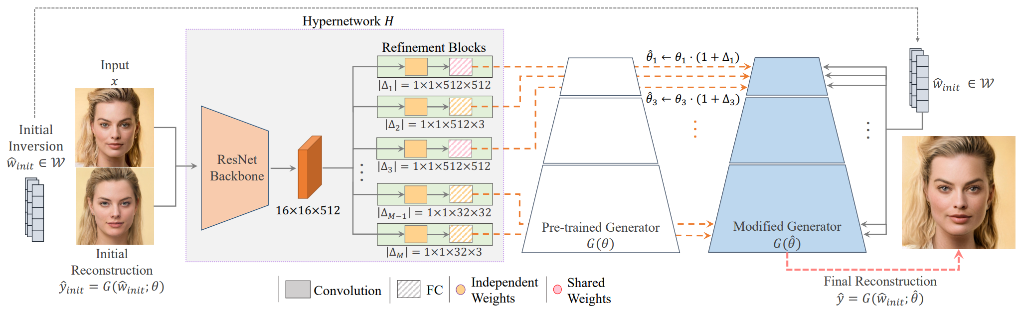
HyperStyle aims to perform ID injection operation by efficiently providing modified weights to the generator as shown in Figure 2 above. We start with image $x$, generator $G$ parameterized with weights $\theta$, and initial inverted latent code $\hat{w}_{init} \in \mathcal{W}$. Using these weights and $\hat{w}_{init}$, the initial reconstructed image $$\hat{y}{init} = G(\hat{w}{init}; \theta)$ create $ A commercial encoder is used to obtain these latent codes.

The goal of this paper is to predict a new set of weights that minimize the objective function for $\hat{\theta}$. To do this, we use the hypernetwork $H$ to predict these weights. We pass both the target image $x$ and the initial coarse image reconstruction $\hat{y}_{init}$ as inputs to help Hypernetwork infer the desired modification.

Therefore, the predicted weight is given by $\hat{\theta} = H(\hat{y}_{init}, x)$. H is trained on a large collection of images to minimize the distortion of the reconstruction.

\[\begin{equation} \sum_{i=1}^N \mathcal{L} (x^i, G (\hat{w}_{init}^i; H (\hat{y}_{init}^i, x^i ))) \end{equation}\]

Given the prediction of the hypernetwork, the final reconstruction can be obtained as $\hat{y} = G(\hat{w}_{init}; \hat{\theta})$.

The initial latent code should be within a well-functioning (i.e. editable) region of the StyleGAN latent space. To do this, we use a pre-trained e4e encoder with $\mathcal{W}$ fixed throughout hypernetwork training. By tweaking these codes, you can apply the same editing techniques used for the original generator.

Indeed, instead of directly predicting the new generator weights, the hypernetwork predicts a set of offsets for the original weights. In addition, by following ReStyle and performing a small number of passes (ex. 5) through hypernetwork, the predicted weight offset is gradually fine-tuned to obtain a higher Creates an inversion of fidelity.

In a sense, HyperStyle can be seen as learning how to optimize generators, but in an efficient way. Also, by learning how to modify the generator, HyperStyle has more freedom to decide how best to project images onto the generator, even when out of bounds. This contrasts with standard encoders, which are limited to encoding into the traditional latent space.

3. Designing the HyperNetwork

StyleGAN generator contains about 30 million parameters. On the one hand, we want the hypernetwork to be expressive and allow us to control these parameters to improve reconstruction. On the other hand, controlling too many parameters results in an inapplicable network, requiring considerable resources to train. Therefore, the design of hypernetworks requires a delicate balance between expressive power and the number of learnable parameters.

$\theta_l = \{\theta_l^{i,j}\}_{i,j = 0}^{C_l^{out}, C_l^{in}} Displayed as$. Here, $\theta_l^{i,j}$ represents the weight of the $j$th channel in the $i$th filter. $C_l^{out}$ represents the total number of filters each including $C_l^{in}$ channels. Letting $M$ be the total number of layers, the generator weight is expressed as $\{\theta_l\}_{l=1}^M$. Hypernetwork creates an offset $\Delta_l$ for each modified layer. These offsets are then multiplied by the corresponding layer weight $\theta_l$ and added to the original weights channel-wise.

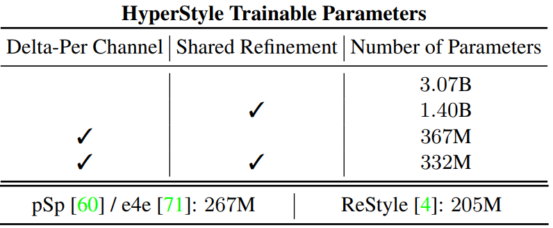
\[\begin{equation} \hat{\theta}_{l}^{i, j} = \theta_l^{i,j} \cdot (1 + \Delta_l^{i,j}) \end{equation}\]

Learning offsets per channel reduces the number of hypernetwork parameters by 88% compared to predicting offsets for each generator parameter.

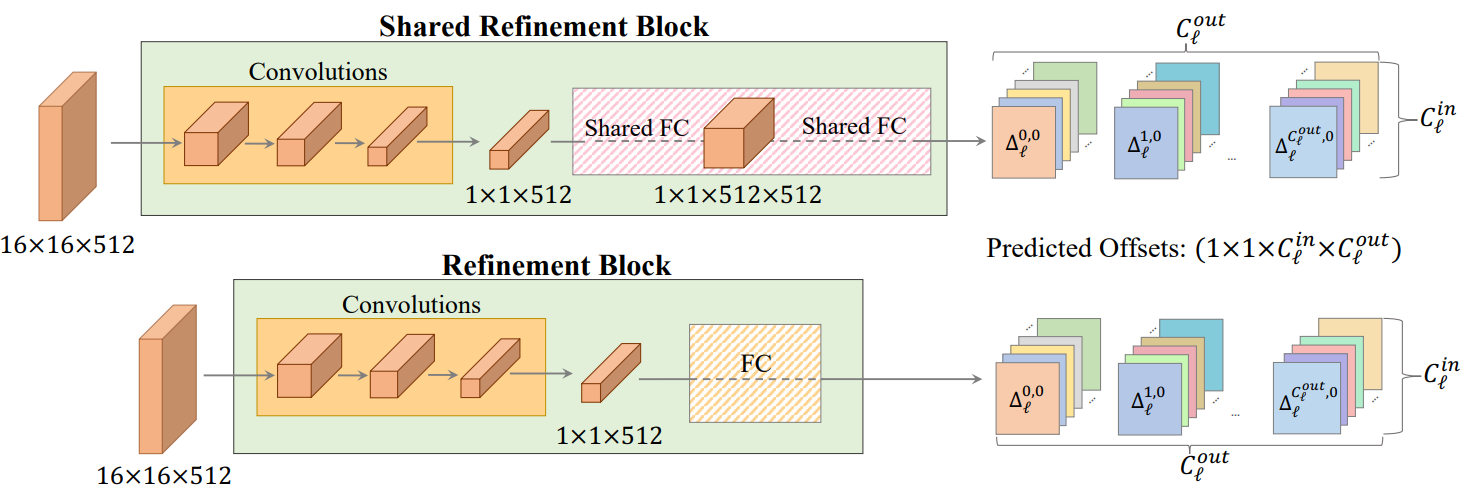
To process the input image, we integrate a ResNet34 backbone that receives 6-channel inputs $x^i, y_{init}^i$ and outputs a 16$\times$16$\times$512 feature map. This shared backbone is followed by a set of refinement blocks, each generating a modulation of a single generator layer. Consider layer $l$ with parameter $\theta_l$ of size $k_l \times k_l \times C_l^{in} \times C_l^{out}$. where $k_l$ is the kernel size. The refinement block receives the feature map extracted from the backbone and outputs an offset of size $1 \times 1 \times C_l^{in} \times C_l^{out}$. Offset is replicated to match the $k_l \times k_l$ kernel dimension of $\theta_l$. Finally, we update the new weights of layer $l$. The Refinement block is explained in the picture above.

To further reduce the number of learnable parameters, we introduce a Shared Refinement Block inspired by the original hypernetwork. These output heads consist of independent convolution layers used to downsample the input feature maps. This is followed by two fully-connected layers shared by multiple generator layers. Here, the weights of the fully-connected layer are shared by the non-toRGB layer of dimension $3 \times 3 \times 512 \times 512$, that is, the largest generator convolutional block. This improves reconstruction quality by allowing information sharing between output heads.

The final configuration, combining Shared Refinement Blocks and per-channel prediction, contains 2.7 billion fewer parameters (~89%) than the naive hypernetwork. The total number of parameters for the various hypernetwork variants is shown in the table below.

Which layers are refined?

Choosing which layer to refine is very important. We can reduce the output dimensionality while focusing the hypernetwork on more meaningful generator weights. Since we invert one ID at a time, any changes to the affine transformation layer are reproduced with each readjustment of the convolution weights. The authors also found that changing the toRGB layer impairs the GAN’s ability to edit. The authors assume that modifying the toRGB layer mainly changes per-pixel textures and colors, with changes that do not translate well in global edits such as poses. Therefore, we limit ourselves to modifying only convolutions, not toRGB.

Finally, we divide the generator layer into three detail levels: coarse, medium, and fine, each controlling a different aspect of the generated image. Early inversions tend to capture coarse details, further limiting the hypernetwork to output offsets for middle and fine generator layers.

To further improve the inversion quality, we adopt the iterative refinement method proposed in Only a Matter of Style thesis. This allows multiple passes through the hypernetwork for a single image inversion. With each step added, the hypernetwork can progressively fine-tune the predicted weight offsets to achieve stronger representation and more accurate inversion.

Perform T passes. For the first pass, use the initial reconstruction $\hat{y}_0 = G(\hat{w}_{init}; \theta)$. For each refinement step $t ≥ 1$, the modified weights $\hat{\theta}t$ and the updated reconstruction $\hat{y}_t = G(\hat{w}_{init}; \hat{ Predict the set of offsets$\Delta_t = H(\hat{y}{t-1}, x)$used to obtain \theta}_t)$. The weight at step $t$ is defined as the accumulated modulation from all previous steps.

\[\begin{equation} \hat{\theta}_{l, t} := \theta \cdot (1 + \sum_{i=1}^t \Delta_{l, i}) \end{equation}\]

The number of refinement steps is set to $T = 5$ during training. Compute the loss at each refinement step. $\hat{w}_{init}$ remains fixed during the iterative process. The final inversion $\hat{y}$ is the reconstruction obtained in the last step.

5. Training Losses

Similar to encoder-based methods, learning proceeds according to the image space reconstruction objective function. We use the weighted sum of the per-pixel $L_2$ loss and the LPIPS perceptual loss. For the face domain, an identity-based similarity loss is additionally applied using a pre-trained face recognition network to preserve face identities. Apply MoCo-based similarity loss for non-face domains. The final loss is:

\[\begin{equation} \mathcal{L}_2 (x, \hat{y}) + \lambda_\textrm{LPIPS} \mathcal{L}_\textrm{LPIPS} (x, \hat{y}) + \lambda_{sim} \ mathcal{L}_{sim} (x, \hat{y}) \end{equation}\]

Experiments

Dataset: FFHQ (train), CelebA-HQ (test), Stanford Cars, AFHQ Wild

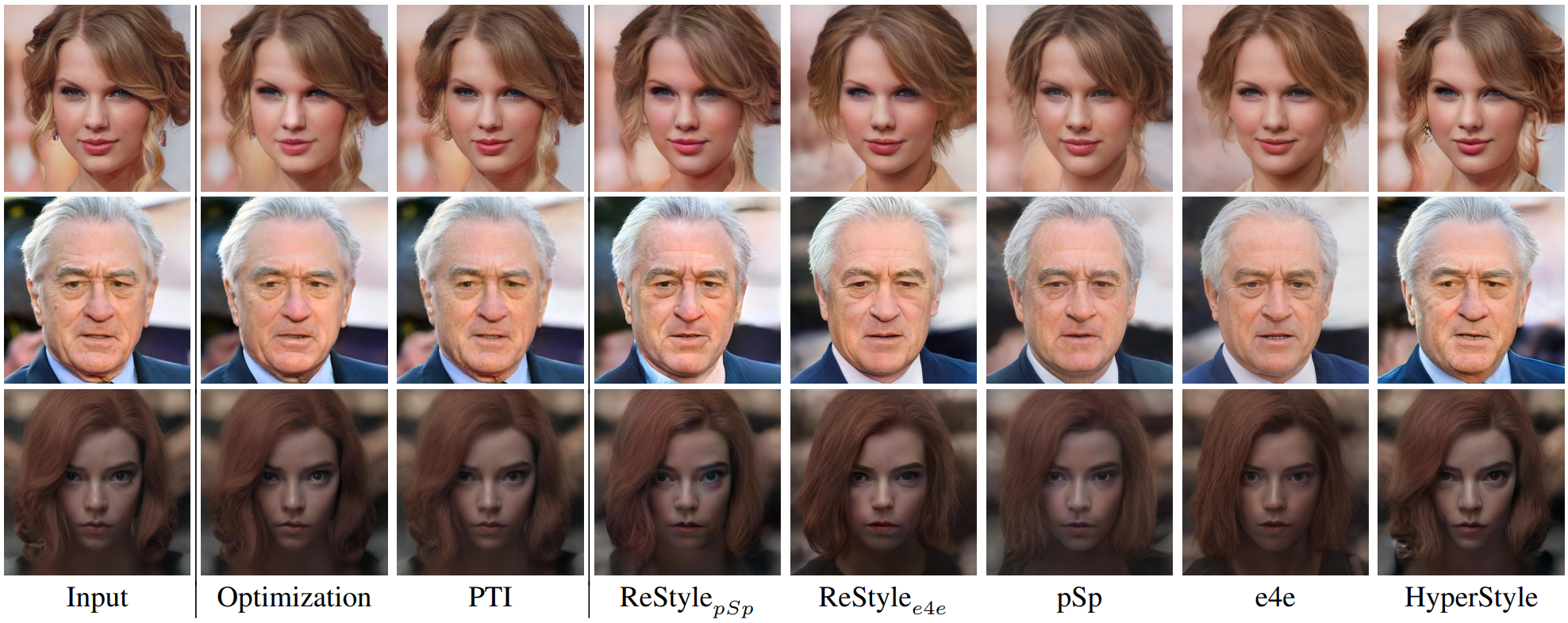
1. Reconstruction Quality

Qualitative Evaluation

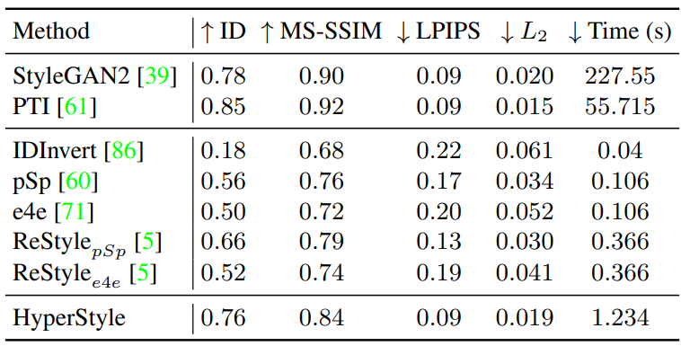
Quantitative Evaluation

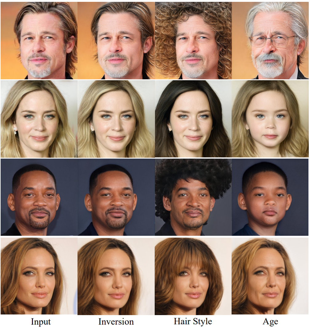
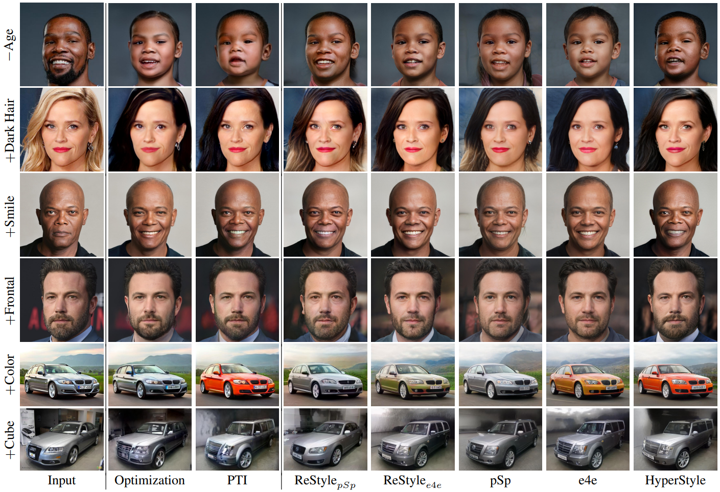
2. Editability via Latent Space Manipulations

Qualitative Evaluation

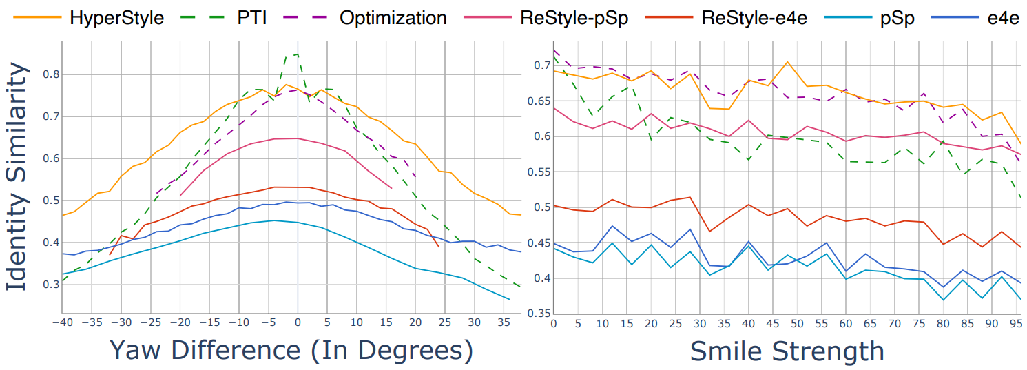
Quantitative Evaluation

3. Ablation Study

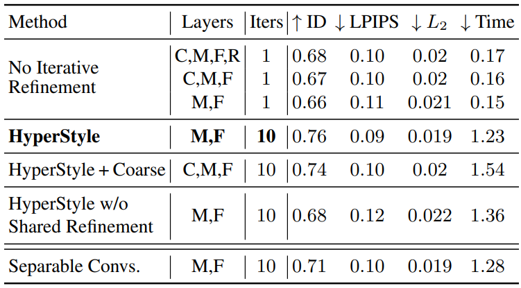
The following table shows the results of the ablation study. Layers C, M, F, and R mean coarse, medium, fine, and toRGB, respectively.

4. Additional Applications

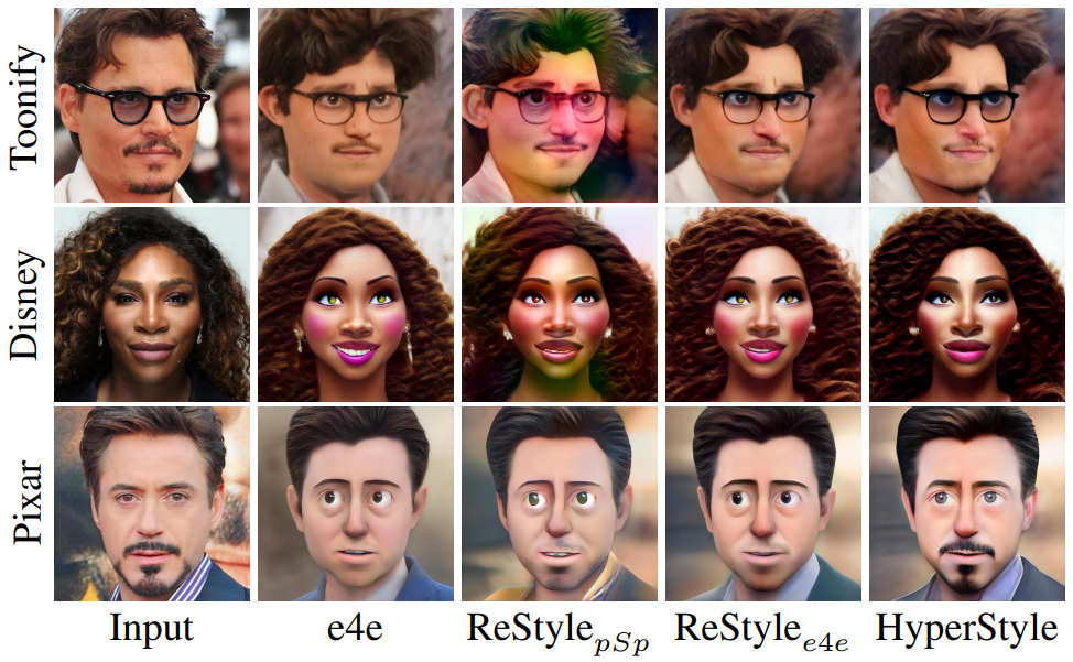
Domain Adaptation

The following is an example of applying the weight offset predicted by HyperStyle learned in FFHQ to modifying a fine-tuned generator (ex. Toonify, StyleGAN-NADA).

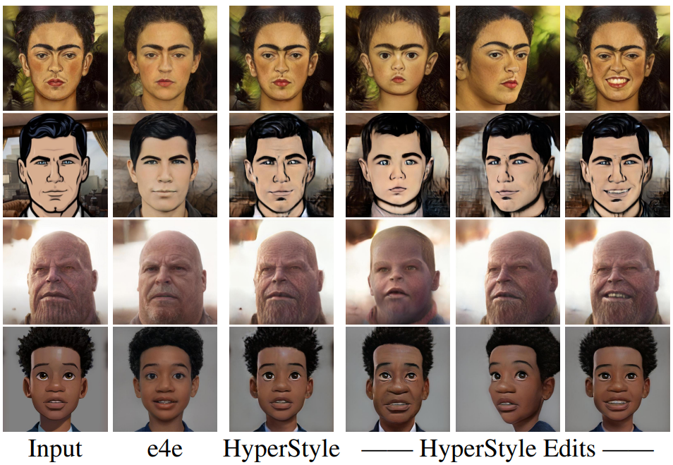
Editing Out-of-Domain Images

This is an example of successfully generalizing a HyperStyle trained only on real images to a tricky style that is not observed during generator fine-tuning training.

Blogs