Blogs

arXiv 2023. [Paper]
David Berthelot, Arnaud Autef, Jierui Lin, Dian Ang Yap, Shuangfei Zhai, Siyuan Hu, Daniel Zheng, Walter Talbott, Eric Gu
Apple
7 Mar 2023

Introduction

Diffusion models are state-of-the-art generative models for many domains and applications. The diffusion model works by learning how to estimate the score of a given data distribution, and in practice it can be implemented as a denoising autoencoder according to a noise schedule. Training a diffusion model is arguably much simpler than many generative modeling approaches such as GANs, normalizing flow, and autoregressive models. Loss is clear and stable, there is considerable flexibility in designing the architecture, and it works directly with continuous inputs without the need for discretization. As shown in recent studies, these properties show excellent scalability for large-scale models and datasets.

Despite empirical success, inference efficiency remains a major challenge for diffusion models. The diffusion model’s inference process can be cast as solving a neural ODE whose sampling quality improves as the discretization error decreases. As a result, up to thousands of denoising steps are actually used to achieve high sampling quality. This dependence on a large number of inference steps disadvantages the diffusion model compared to one-shot sampling methods such as GANs, especially in resource-constrained cases.

Existing efforts to speed up the inference of diffusion models can be classified into three classes.

1. Reduce input dimensionality
2. Improved ODE solver
3. Gradual distillation

Among these, the gradual distillation method aroused the authors’ interest. Using a DDIM inference schedule takes advantage of the fact that there is a deterministic mapping between the initial noise and the final generated result. Through this, it is possible to learn an efficient student model that is close to the given teacher model. A naive implementation of this distillation is forbidden because it requires calling the teacher network $T$ (if $T$ is usually large) for each student network update. Paper Progressive distillation for fast sampling of diffusion models circumvents this problem by performing Progressive Binary Time Distillation (BTD). In BTD, distillation is divided into $\log_2 (T)$ phases, and in each phase, the student model learns the inference result of two consecutive teacher models. Experimentally, BTD can reduce inference steps to 4 with little performance loss on CIFAR-10 and 64$\times$64 ImageNet.

In this paper, we aim to raise the inference efficiency of the diffusion model to the limit. In other words, we aim for one-step inference using high-quality samples. First, we identify significant drawbacks of BTD that prevent it from achieving this goal.

1. Approximation errors accumulate from one distillation phase to the next, causing the objective function to degenerate.
2. Since the learning process is divided into $\log_2 (T)$ phases, we avoid using aggressive stochastic weights averaging (SWA) to achieve good generalization.

Motivated by these observations, we propose a new diffusion model distillation method called TRAnsitive Closure Time-Distillation (TRACT). Briefly, TRACT trains the student model and extracts the inference output of the teacher model from step $t$ to step $t’$ where $t’ < t$. To obtain $t \rightarrow t - 1$, one step inference update of the teacher model is performed, and then the objective function is calculated by calling the student model to obtain $t - 1 \rightarrow t’$ by bootstrapping method. After distillation, one-step inference can be performed with the teacher model by setting $t = T$ and $t’ = 0$. The authors avoid BTD’s objective function regression and SWA incompatibility by showing that TRACT can be trained in only one or two phases.

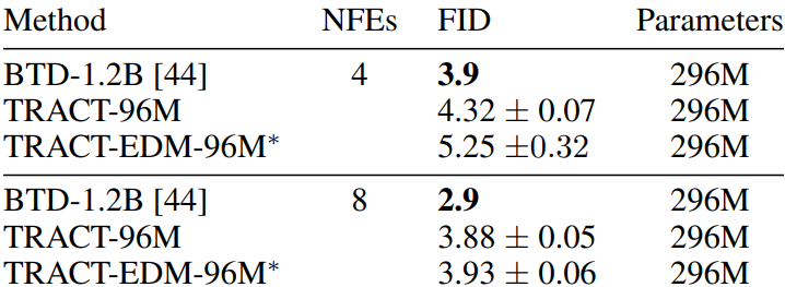
The authors experimentally confirmed that TRACT significantly improves state-of-the-art results with one-step and two-step inference. In particular, we achieved one-step FID scores of 7.4 and 3.8 for 64$\times$64 ImageNet and CIFAR10, respectively.

Background

DDIMs

DDIM uses the $T$-step noise schedule $\gamma_t \in [0, 1)$, where $t = 0$ is a noiseless step and $\gamma_0 = 1$. In the variance preserving (VP) setting, the noisy sample $x_t$ is generated with the original sample $x_0$ and the Gaussian noise $\epsilon$.

\[\begin{equation} x_t = x_0 \sqrt{\gamma_t} + \epsilon \sqrt{1 - \gamma_t} \end{equation}\]

The neural network f_\theta$ is trained to predict signal or noise, or both. The estimated values of $x_0$ and $\epsilon$ of each step $t$ are expressed as $x_{0 \vert t}$ and $\epsilon_{\vert t}$. For brevity, only the signal prediction case is described. In the denoisification phase, $\epsilon_{\vert t}$ is estimated using $x_{0 \vert t}$ predicted by the following equation.

\[\begin{equation} x_{0 \vert t} := f_\theta (x_t, t), \quad \epsilon_{\vert t} = \frac{x_t - x_{0 \vert t} \sqrt{\gamma_t}}{\sqrt{1 - \gamma_t}} \end{equation}\]

With this estimation, inference is possible.

\[\begin{aligned} x_{t'} &= \delta (f_\theta, x_t, t, t') \\ & := x_t \frac{\sqrt{1 - \gamma_{t'}}}{\sqrt{1 - \gamma_t}} + f_\theta (x_t, t) \frac{\sqrt{\gamma_{t'} (1-\gamma_t)} - \sqrt{\gamma_t (1 - \gamma_{t'})}}{\sqrt{1 - \gamma_t}} \end{aligned}\]

Here, the step function $\delta$ is the DDIM inference from $x_t$ to $x_{t’}$.

Binary Time Distillation (BTD)

Student network $g_\phi$ is trained to alternate 2 denoising steps of teacher $f_\theta$.

\[\begin{equation} \delta (g_\phi, x_t, t, t-2) \approx x_{t-2} := \delta (f_\theta, \delta (f_\theta, x_t, t, t-1), t- 1, t-2) \end{equation}\]

According to this definition, target $\hat{x}$ that satisfies the above equation can be obtained.

\[\begin{equation} \hat{x} = \frac{x_{t-2} \sqrt{1 - \gamma_t} - x_t \sqrt{1 - \gamma_{t-2}}}{\sqrt{\gamma_{t-2} } \sqrt{1 - \gamma_t} - \sqrt{\gamma_t} \sqrt{1 - \gamma_{t-2}}} \end{equation}\]

We can rewrite the loss as the noise prediction error as

\[\begin{equation} \mathcal{L} (\phi) = \frac{\gamma_t}{1 - \gamma_t} \| g_\phi (x_t, t) - \hat{x} \|_2^2 \end{equation}\]

If the student trains to completion, then becomes the teacher, and the process is repeated until the final model has the desired number of steps. It takes $\log_2 T$ training phases to distill a $T$-step teacher into a one-step model, and each trained student needs half of the teacher’s sampling steps to generate a high-quality sample.

Method

This paper proposes TRansitive Closure Time-Distillation (TRACT), an extension of BTD that reduces the number of distillation phases from $\log_2 T to a small constant (usually 1 or 2). We first focus on the VP settings used in BTD, but the method itself is independent of it and is available in Variance Exploding (VE) settings. TRACT works for the noise prediction objective, but also for signal prediction where the neural network predicts an estimate of $x_0$.

1. Motivation

The authors speculate that the final quality of the sample in the distilled model is influenced by the number of distillation phases and the length of each phase. Consider two potential explanations for why.

Objective degeneracy

In BTD, the student of the previous distillation phase becomes the teacher of the next phase. A student in a previous phase has a positive loss resulting in an incomplete teacher in the next phase. These imperfections accumulate over successive generations of teachers, leading to regression of the objective function.

Generalization

Stochastic Weight Averaging (SWA) was used to improve the performance of neural networks trained for DDPM. With Exponential Moving Average (EMA), the momentum parameter is limited by the learning length. High momentum yields high-quality results, but too short a training length leads to over-regularized models. This is related to the time distillation problem because the total learning length is directly proportional to the number of learning phases.

2. TRACT

TRACT is a multi-phase method in which each phase distills the $T$-step schedule to $T’ < T$ step and repeats until the desired number of steps is reached. In a phase, the $T$-step schedule is divided into $T’$ contiguous groups. Any partitioning strategy can be used. For example, the experiment used groups of the same size as in Algorithm 1.

The method in this paper can be seen as an extension of BTD that is not limited by $T’ = T/2$. However, relaxation of this constraint makes computational sense, such as estimating $x_t’$ from $x_t$ for $t’ < t$.

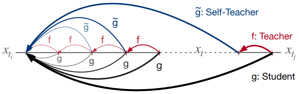
For the continuous segments \(\{t_i, \cdots, t_j\}\), model student $g_\phi$ to jump from any step $t_i < t \le t_j$ to step $t_i$ as shown in the figure above. do.

\[\begin{equation} \delta (g_\phi, x_t, t, t_i) = \delta (f_\theta, \delta (f_\theta, \cdots, \delta (f_\theta, x_t, t, t-1), \cdots) , t_{i+1}, t_i) \end{equation}\]

Student $g$ is specified to include the denoising step $(t_j - t_i)$ of $f$. However, this formula can be very computationally expensive as $f$ must be called multiple times during training.

To solve this problem, we use self-teacher whose weight is the EMA of student $g$. This approach is inspired by semi-supervised learning, reinforcement learning, and representation learning. For the student network $g$ with weight $\phi$, the EMA of the weight is expressed as $\tilde{\phi} = \textrm{EMA} (\phi, \mu_S)$. Here, the momentum $\mu_S \in [0, 1] $ is a hyper-parameter.

Therefore, the transitive closure operator can be modeled as self-teaching by rewriting the above equation.

\[\begin{equation} \delta (g_\phi, x_t, t, t_i) \approx x_{t_i} := \delta (g_{\tilde{\phi}}, \delta (f_\theta, x_t, t, t-1), t-1, t_i) \end{equation}\]

From this definition, we can determine the target $\hat{x}$ that satisfies the equation.

\[\begin{equation} \hat{x} = \frac{x_{t_i} \sqrt{1 - \gamma_t} - x_t \sqrt{1 - \gamma_{t_i}}}{\sqrt{\gamma_{t_i}} \sqrt{1 - \gamma_t} - \sqrt{\gamma_t} \sqrt{1 - \gamma_{t_i}}} \end{equation}\]

If $t_i = t-1$, then $\hat{x} = f_\theta (x_t, t)$.

The loss for $\hat{x}$ is

\[\begin{equation} \mathcal{L} (\phi) = \frac{\gamma_t}{1 - \gamma_t} \| g_\phi (x_t, t) - \hat{x} \|_2^2 \end{equation}\]

3. Adapting TRACT to a Runge-Kutta teacher and Variance Exploding noise schedule

To demonstrate generality, TRACT is applied to teachers of Elucidating the Design space of diffusion Model (EDM) using VE noise schedule and RK sampler.

VE noise schedules

VE noise schedule is for \(t \in \{1, \cdots, T\}\) where \(\sigma_1 = \sigma_{min} \le \sigma_t \le \sigma_T = \sigma_{max}\) It is parameterized as a series of noise standard deviations $\sigma_t \ge 0$, where t = 0 represents a noiseless step \sigma_0 = 0$. The noisy sample $x_t$ is generated from the original sample $x_0$ and the Gaussian noise $\epsilon$ as follows.

\[\begin{equation} x_t = x_0 + \sigma_t \epsilon \end{equation}\]

RK step function

Following the EDM approach, we use the RK sampler as the teacher and distill the DDIM sampler as the student. Step functions are $\delta_{RK}$ and $\delta_{DDIM-VE}$, respectively. The $\delta_{RK}$ step function ($t > 0$) estimating $x_t’$ from $x_t$ is defined as:

\[\begin{equation} \delta_{RK} (f_\theta, x_t, t, t') := \begin{cases} x_t + (\sigma_{t'} - \sigma_t) \epsilon (x_t, t) & \textrm{if } t' = 0 \\ x_t + \frac{1}{2} (\sigma_{t'} - \sigma_t) [\epsilon (x_t, t) + \epsilon (x_t + (\sigma_{t'} - \sigma_t) \epsilon (x_t, t), t)] & \textrm{otherwise} \end{cases} \\ \textrm{where} \quad \epsilon (x_t, t) := \frac{x_t - f_\theta (x_t, t)}{\sigma_t} \end{equation}\]

The $\delta_{DDIM-VE}$ step function that estimates $x_{t’}$ from $x_t$ is defined as follows.

\[\begin{equation} \delta_{DDIM-VE} (f_\theta, x_t, t, t') := f_\theta (x_t, t) \bigg( 1 - \frac{\sigma_{t'}}{\sigma_t} \bigg ) + \frac{\sigma_{t'}}{\sigma_t} x_t \end{equation}\]

Then, to learn the transitive closure operator through self-teaching, the following equation is required.

\[\begin{equation} \delta_{DDIM-VE} (f_\theta, x_t, t, t') \approx x_{t_i} := \delta_{DDIM-VE} (g_{\tilde{\phi}}, \delta_{RK} (f_\theta, x_t, t, t-1), t-1, t_i) \end{equation}\]

From this definition, we can determine the target $\hat{x}$ that satisfies the equation.

\[\begin{equation} \hat{x} = \frac{\sigma_t x_{t_i} - \sigma_{t_i} x_t}{\sigma_t - \sigma_{t'}} \end{equation}\]

Then the loss is the weighted loss between the student network’s prediction and $\hat{x}$.

\[\begin{equation} \mathcal{L}(\phi) = \lambda (\sigma_t) \| g_\phi (x_t, t) - \hat{x} \|_2^2 \end{equation}\]

Experiment

1. Image generation results

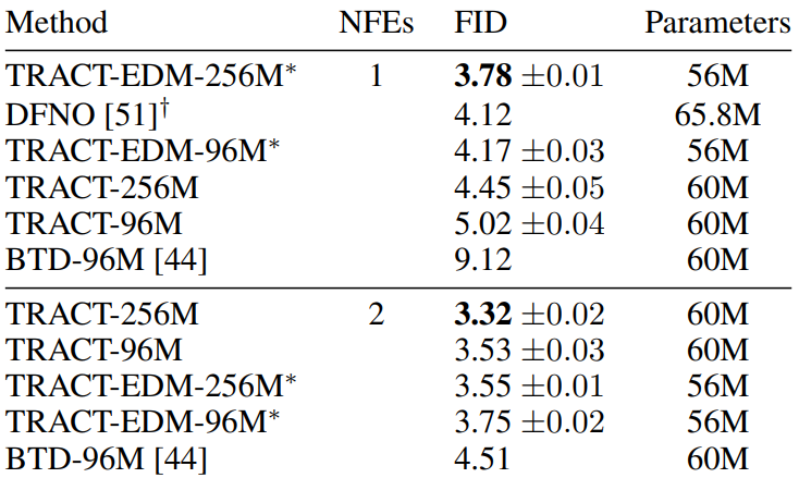
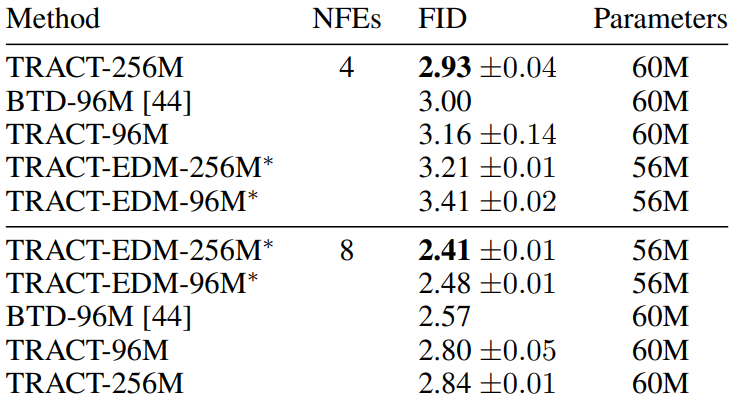
CIFAR-10

The following is a table showing the FID results in CIFAR-10.

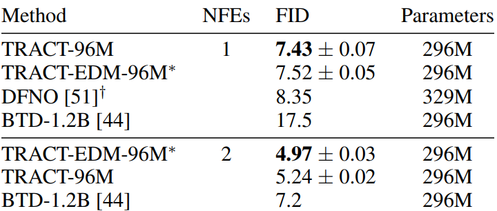
64$\times$64 ImageNet

The following table shows the FID results on 64$\times$64 ImageNet.

2. Stochastic Weight Averaging Ablations

The authors used a bias-corrected EMA in their experiments.

\[\begin{aligned} \tilde{\phi}_0 &= \phi_0 \\ \tilde{\phi}_i &= \bigg(1 - \frac{1 - \mu_S}{1 - \mu_S^i} \bigg) \tilde{\phi}_{i-1} + \frac{1 - \mu_S}{1 - \mu_S^i} \phi_i \end{aligned}\]

In the ablation study, the distillation schedule was fixed at $1024 \rightarrow 32 \rightarrow 1$, and 48 million samples were used per phase.

Self-teaching EMA

The following is the result of performing an ablation study on $\mu_S$ with $\mu_I = 0.99995$ fixed. (CIFAR-10)

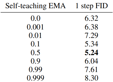
It can be seen that the value of $\mu_S$ shows good performance in a wide range.

Inference EMA

This is the result of fixing $\mu_S = 0.5$ and conducting an ablation study on $\mu_I$. (CIFAR-10)

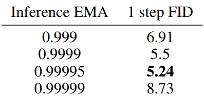
It can be seen that the value of $\mu_I$ has a great effect on performance.

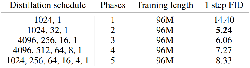
3. Influence of the number of distillation phases

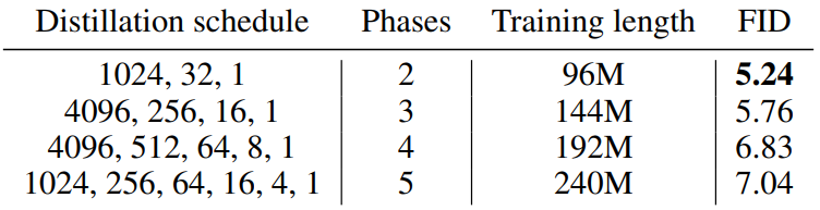
Fixed overall training length

The following is the ablation result when the total learning length is fixed.

Fixed training length per phase

The following is the ablation result when the learning length per phase is fixed.

Binary Distillation comparison

The authors compared BTD to TRACT on the same BTD-compatible schedule ($1024 \rightarrow 512 \rightarrow \cdots \rightarrow 2 \rightarrow 1$) to further confirm that objective function regression is why TRACT outperforms BTD. Both experiments set $\mu_I = 0.99995 $ and used 48 million samples per phase. In this setup, BTD’s FID is 5.95, TRACT’s FID is 6.8, and BTD outperforms TRACT. This further confirms that the poor overall performance of BTD may be due to its inability to utilize the 2-phase schedule.

Besides schedule, the difference between BTD and TRACT is TRACT’s use of self-teaching. This experiment also suggests that self-teaching training may result in a less efficient objective function than supervised learning.