


NeurIPS 2020. [Paper] [Github]
Jonathan Ho, Ajay Jain, Pieter Abbeel
UC Berkeley
19 Jun 2020
Introduction
This thesis is an advanced thesis of the diffusion model. Diffusion model is a model that trains a parameterized Markov chain to create samples that fit the desired data after a finite time. In the forward process, the Markov chain gradually adds noise to finally make Gaussian noise. Conversely, the reverse process gradually removes the noise from the Gaussian noise, finally creating samples that fit the desired data. Since the diffusion consists of a small amount of Gaussian noise, it is sufficient to set the sampling chain to a conditional Gaussian, and it can be parameterized with a simple neural model.
Existing diffusion models are easy to define and efficient to train, but do not produce high-quality samples. On the other hand, DDPM not only made high-quality samples, but also showed better results than other generative models (eg GAN). In addition, we show that the specific parameterization of the diffusion model is comparable to denoising score matching at various noise levels during training and equivalent to solving the Langevin dynamics problem during sampling.
Among other features
- DDPM produces high-quality samples, but it does not have log likelihood that is competitive with other likelihood-based models.
- DDPM’s lossless codelength was used to describe mostly imperceptible image details.
- It was shown that the sampling of the diffusion model is a progressive decoding similar to that of the autoregressive model.
Diffusion model
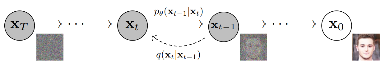
The diffusion model is defined as $p_\theta (x_0) := \int p_\theta (x_{0:T}) dx_{1:T}$. $x_1, \cdots, x_T$ are the same size as the data $x_0 \sim q(x_0 )$. Joint distribution $p_\theta (x_{0:T})$ is called the reverse process, and it is a Gaussian transition starting from $p(x_T ) = \mathcal{N} (x_T ; 0, I )$. It is defined as a Markov chain consisting of
\[\begin{equation} p_\theta (x_{0:T}) := p(x_T) \prod_{t=1}^T p_\theta (x_{t-1}|x_{t}) \\ p_\theta (x_{t-1}|x_{t}) := \mathcal{N} (x_{t-1} ; \mu_\theta (x_t , t), \Sigma_\theta (x_t , t) ) \end{equation}\]
The difference between the diffusion model and other latent variable models is that the approximate posterior $q(x_{1:T}|x_0)$ called the forward process or diffusion process It is a Markov chain that gradually adds Gaussian noise according to $\beta_1, \cdots, and \beta_T$.
Learning proceeds by optimizing a general variational bound for the negative log likelihood.
\[\begin{equation} L:= \mathbb{E} [-\log p_\theta (x_0)] \le \mathbb{E}_q \bigg[ -\log \frac{p_\theta (x_{0:T})}{q (x_{1:T}|x_0)} \bigg] \le \mathbb{E}_q \bigg[ -\log p(x_T) - \sum_{t \ge 1} \log \frac{p_\theta (x_{t-1}|x_t)}{q(x_t |x_{t-1})} \bigg] \end{equation}\]$\beta_t$ can be trained with reparameterization or kept constant as a hyper-parameter. Also, if $\beta_t$ is sufficiently small, the expressiveness of the reverse process is This is partially guaranteed by the choice of the Gaussian conditional at $p_\theta (x_{t-1}|x_t)$.
What is noteworthy about the forward process is that sampling $x_t$ is possible at any time $t$ in closed form.
\[\begin{equation} \alpha_t := 1-\beta_t, \quad \bar{\alpha_t} := \prod_{s=1}^t \alpha_s \\ q(x_t | x_0) = \mathcal{N} (x_t ; \sqrt{\vphantom{1} \bar{\alpha_t}} x_0 , (1-\bar{\alpha_t})I) \end{equation}\]Proof)
Since $q (x_{t}|x_{t-1}) = \mathcal{N} (x_{t} ; \sqrt{1-\beta_t} x_{t-1}, \beta_t I)$ $$ \begin{aligned} x_t &= \sqrt{1-\beta_t} x_{t-1} + \sqrt{\beta_t} \epsilon_{t-1} & (\epsilon_{t-1} \sim \mathcal{N} (0, I)) \\ &= \sqrt{\alpha_t} x_{t-1} + \sqrt{1-\alpha_t} \epsilon_{t-1} \\ &= \sqrt{\alpha_t} (\sqrt{\alpha_{t-1}} x_{t-2} + \sqrt{1-\alpha_{t-1}} \epsilon_{t-2}) + \ sqrt{1-\alpha_t} \epsilon_{t-1} & (\epsilon_{t-2} \sim \mathcal{N}(0, I))\\ &= \sqrt{\alpha_t \alpha_{t-1}} x_{t-2} + \sqrt{\alpha_t (1-\alpha_{t-1})} \epsilon_{t-2} + \sqrt{ 1-\alpha_t} \epsilon_{t-1} \\ \end{aligned} $$ $\alpha_t (1-\alpha_{t-1}) + 1-\alpha_t = 1 - \alpha_t \alpha_{t-1}$ so $\sqrt{\alpha_t (1-\alpha_{t-1}) } \epsilon_{t-2} + \sqrt{1-\alpha_t} \epsilon_{t-1} \sim \mathcal{N}(0, (1 - \alpha_t \alpha_{t-1})I)$ and substituting, $$ \begin{aligned} x_t &= \sqrt{\alpha_t \alpha_{t-1}} x_{t-2} + \sqrt{1 - \alpha_t \alpha_{t-1}} \epsilon'_{t-2} & (\ epsilon'_{t-2} \sim \mathcal{N}(0, I)) \\ &= \sqrt{\alpha_t \alpha_{t-1} \alpha_{t-2}} x_{t-3} + \sqrt{1 - \alpha_t \alpha_{t-1} \alpha_{t-2} } \epsilon'_{t-3} & (\epsilon'_{t-3} \sim \mathcal{N}(0, I)) \\ &= \cdots \\ &= \sqrt{ \vphantom{1} \bar{\alpha}_t} x_{0} + \sqrt{1 - \bar{\alpha}_t} \epsilon'_{0} & (\epsilon'_{ 0} \sim \mathcal{N}(0, I)) \end{aligned} $$
Thus, $q(x_t | x_0) = \mathcal{N} (x_t ; \sqrt{\vphantom{1} \bar{\alpha}_t} x_0 , (1-\bar{\alpha}_t)I)$ am.
Since sampling is possible at one time, efficient learning is possible using stochastic gradient descent. A further improvement is possible due to reduced variance by rewriting $L$ as:
The equation above directly compares the forward process posterior (ground truth) with $p_\theta (x_{t-1} \vert x_t)$ as the KL divergence, which is tractable. Since the KL divergence for two Gaussian distributions can be calculated by the Rao-Blackwellized method in closed form, $L$ can be calculated easily.
$q(x_{t-1} \vert x_t, x_0)$ can be calculated as follows.
\[\begin{aligned} q (x_{t-1} | x_t, x_0) &= \mathcal{N} (x_{t-1} ; \tilde{\mu_t} (x_t, x_0), \tilde{\beta_t} I), \\ \rm{where} \quad \tilde{\mu_t} (x_t, x_0) &:= \frac{\sqrt{\vphantom{1} \bar{\alpha}_{t-1}} \beta_t}{1-\bar{\alpha}_t} x_0 + \frac{\sqrt{\alpha_t}(1-\bar{\alpha}_{t-1})}{1-\bar{\alpha}_t} x_t \quad \rm{and} \quad \tilde{\beta_t} := \frac{1-\bar{\alpha}_{t-1}}{1-\bar{\alpha}_t} \beta_t \end{aligned}\]Proof)
$$ \begin{aligned} q(x_{t-1} | x_t, x_0) &= q(x_t | x_{t-1}, x_0) \frac{q(x_{t-1} | x_0)}{q(x_t | x_0)} \\ & \propto \exp \bigg(- \frac{1}{2} (\frac{(x_t - \sqrt{\alpha_t} x_{t-1})^2}{\beta_t} + \frac{(x_{t-1} - \sqrt{\vphantom{1} \bar{\alpha}_{t-1}} x_0)^2}{1-\bar{\alpha}_{t-1}} - \frac{(x_t - \sqrt{\vphantom{1} \bar{\alpha}_{t}} x_0)^2}{1-\bar{\alpha}_{t}}) \bigg) \\ &= \exp \bigg(- \frac{1}{2} (\frac{x_t^2 - 2\sqrt{\alpha_t} x_t x_{t-1} + \alpha_t x_{t-1}^2}{\beta_t} + \frac{x_{t-1}^2 - 2\sqrt{\vphantom{1} \bar{\alpha}_{t-1}} x_{t-1} x_0 + \bar{\alpha}_{t-1} x_0^2}{1-\bar{\alpha}_{t-1}} - \frac{(x_t - \sqrt{\vphantom{1} \bar{\alpha}_{t}} x_0)^2}{1-\bar{\alpha}_{t}}) \bigg) \\ &= \exp \bigg(- \frac{1}{2} ((\frac{\alpha_t}{\beta_t} + \frac{1}{1-\bar{\alpha}_{t-1}}) x_{t-1}^2 - 2(\frac{\sqrt{\alpha_t}}{\beta_t}x_t + \frac{\sqrt{\vphantom{1} \bar{\alpha}_{t-1}}}{1-\bar{\alpha}_{t-1}} x_0) x_{t-1} + C(x_t, x_0)) \bigg) \\ &= A(x_t, x_0) \exp \bigg( -\frac{1}{2 \tilde{\beta}_t} (x_{t-1} - \tilde{\mu}_t (x_t, x_0))^2 \bigg) \\ \tilde{\beta}_t &= 1 / \bigg( \frac{\alpha_t}{\beta_t} + \frac{1}{1-\bar{\alpha}_{t-1}} \bigg) = \frac{\beta_t (1-\bar{\alpha}_{t-1})}{\alpha_t (1-\bar{\alpha}_{t-1}) + \beta_t} = \frac{\beta_t (1-\bar{\alpha}_{t-1})}{\alpha_t -\alpha_t \bar{\alpha}_{t-1} + \beta_t} = \frac{1-\bar{\alpha}_{t-1}}{1 - \bar{\alpha}_t} \beta_t \\ \tilde{\mu_t} (x_t, x_0) &= (\frac{\sqrt{\alpha_t}}{\beta_t}x_t + \frac{\sqrt{\vphantom{1} \bar{\alpha}_{t-1}}}{1-\bar{\alpha}_{t-1}} x_0) \tilde{\beta}_t = (\frac{\sqrt{\alpha_t}}{\beta_t}x_t + \frac{\sqrt{\vphantom{1} \bar{\alpha}_{t-1}}}{1-\bar{\alpha}_{t-1}} x_0) \frac{1-\bar{\alpha}_{t-1}}{1 - \bar{\alpha}_t} \beta_t \\ &= \frac{\sqrt{\vphantom{1} \bar{\alpha}_{t-1}} \beta_t}{1-\bar{\alpha}_t} x_0 + \frac{\sqrt{\alpha_t}(1-\bar{\alpha}_{t-1})}{1-\bar{\alpha}_t} x_t \end{aligned} $$
As above, $q(x_{t-1} \vert x_t)$ is difficult to compute, but $q(x_{t-1} \vert x_t, x_0)$ is easy to compute. In other words, it is difficult to directly obtain $x_{t-1}$ from $x_t$, but it can be obtained easily by giving $x_0$ as a condition.
Diffusion models and denoising autoencoders
1. Forward process and $L_T$
Since we will fix the variance $\beta_t$ of the forward process as a constant in the experiment, there are no parameters to be learned in the approximate posterior $q$. Therefore, during training, $L_T$ is a constant and can be ignored.
2. Reverse process and $L_{1:T-1}$
$p_\theta (x_{t-1} \vert x_t) = \mathcal{N} (x_{t-1} ; \mu_\theta (x_t, t) ; \Sigma_ for $1 < t \le T$ \theta (x_t, t))$ is set as follows.
- $\Sigma_\theta (x_t, t) = \sigma_t^2 I$, and $\sigma_t$ is a constant that depends on $t$ that is not learned. As a result of experiments, it is said that $\sigma_t^2 = \beta_t$ or $\sigma_t^2 = \tilde{\beta_t}$ gives similar results.
- We propose a specific parameterization to represent $\mu_\theta (x_t, t)$. For $p_\theta (x_{t-1}\vert x_t) = \mathcal{N} (x_{t-1} ; \mu_\theta (x_t, t), \sigma_t^2 I)$ can be written together
proof)
If $q(x) = \mathcal{N} (\mu_1, \sigma_1^2)$ and $p(x) = \mathcal{N} (\mu_2, \sigma_2^2)$ then the KL divergence is same. $$ \begin{equation} D_{KL} (q \| p) = - \int q(x) \log p(x) dx + \int q(x) \log q(x) dx \end{equation} $$ $$ \begin{aligned} - \int q(x) \log p(x) dx &= - \int q(x) \log \frac{1}{(2\pi \sigma_2^2)^{(1/2)}} e^{- \frac{(x-\mu_2)^2}{2\sigma_2^2}} dx \\ &= \frac{1}{2} \log (2\pi \sigma_2^2) - \int q(x) \bigg( - \frac{(x-\mu_2)^2}{2\sigma_2^2} \bigg) dx \\ &= \frac{1}{2} \log (2\pi \sigma_2^2) + \frac{\int q(x) x^2 dx - \int q(x) 2x\mu_2 dx + \int q(x)\mu_2^2 dx}{2\sigma_2^2} \\ &= \frac{1}{2} \log (2\pi \sigma_2^2) + \frac{\langle x^2 \rangle - 2\langle x \rangle \mu_2 + \mu_2^2}{2\sigma_2^2} \\ &= \frac{1}{2} \log (2\pi \sigma_2^2) + \frac{\sigma_1^2 + \mu_1^2 - 2 \mu_1 \mu_2 + \mu_2^2}{2\sigma_2^2} \\ &= \frac{1}{2} \log (2\pi \sigma_2^2) + \frac{\sigma_1^2 + (\mu_1 - \mu_2)^2}{2\sigma_2^2} \\ \end{aligned} $$ $$ \begin{aligned} D_{KL} (q \| p) &= \frac{1}{2} \log (2\pi \sigma_2^2) + \frac{\sigma_1^2 + (\mu_1 - \mu_2)^2}{2\sigma_2^2} - \frac{1}{2} \log (2\pi \sigma_1^2) - \frac{1}{2} \\ &= \frac{1}{2} \log ( \frac{\sigma_2^2}{\sigma_1^2}) + \frac{\sigma_1^2 - \sigma_2^2 + (\mu_1 - \mu_2)^2}{2\sigma_2^2} \\ \end{aligned} $$ $q (x_{t-1} \vert x_t, x_0) = \mathcal{N} (x_{t-1} ; \tilde{\mu_t} (x_t, x_0), \tilde{\beta_t} I)$이고 $p_\theta (x_{t-1} \vert x_t) = \mathcal{N} (x_{t-1} ; \mu_\theta (x_t, t), \sigma_t^2 I)$이므로 $\mu_1 = \tilde{\mu_t} (x_t, x_0)$, $\mu_2 = \mu_\theta (x_t, t)$, $\sigma_1^2 = \tilde{\beta_t}$, $\sigma_2^2 = \sigma_t^2$를 $L_{t-1}$에 대입하면 다음과 같다. $$ \begin{aligned} L_{t-1} &= \mathbb{E}_q \bigg[ D_{KL} (q(x_{t-1} | x_t , x_0) \; || \; p_\theta (x_{t-1} | x_t)) \bigg] \\ &= \mathbb{E}_q \bigg[ \frac{1}{2} \log ( \frac{\sigma_t^2}{\tilde{\beta_t}}) + \frac{\tilde{\beta_t} - \sigma_t^2 + (\tilde{\mu_t} (x_t, x_0) - \mu_\theta (x_t, t))^2}{2\sigma_t^2} \bigg]\\ &= \mathbb{E}_q \bigg[ \frac{\tilde{\beta_t} - \sigma_t^2 + (\tilde{\mu_t} (x_t, x_0) - \mu_\theta (x_t, t))^2}{2\sigma_t^2} \bigg] + \mathbb{E}_q \bigg[ \frac{1}{2} \log ( \frac{\sigma_t^2}{\tilde{\beta_t}}) + \frac{\tilde{\beta_t} - \sigma_t^2}{2\sigma_t^2}\bigg] \\ &= \mathbb{E}_q \bigg[ \frac{1}{2\sigma_t^2} \| \tilde{\mu_t} (x_t, x_0) - \mu_\theta (x_t, t) \|^2 \bigg] + C \\ \end{aligned} $$ $C$ is a value calculated from $\tilde{\beta_t}$ and $\sigma_t^2$, so it depends only on $t$.
$C$ is a constant independent of $\theta$. Therefore, $L_{t-1}$ is learned so that $\mu_\theta$ approaches the ground truth $\tilde{\mu_t}$. the sampling expression
If you transform
\[\begin{equation} x_0 = \frac{1}{\sqrt{\vphantom{1} \bar{\alpha}_t}} (x_t(x_0, \epsilon) - \sqrt{1-\bar{\alpha}_t}\epsilon) \end{equation}\]and substituting it into $\tilde{\mu_t} (x_t, x_0)$, we get the following.
\[\begin{aligned} \tilde{\mu_t} (x_t, x_0) &= \frac{\sqrt{\vphantom{1} \bar{\alpha}_{t-1}} \beta_t}{1-\bar{\alpha}_t} x_0 + \frac{\sqrt{\alpha_t}(1-\bar{\alpha}_{t-1})}{1-\bar{\alpha}_t} x_t \\ &= \frac{\sqrt{\vphantom{1} \bar{\alpha}_{t-1}} \beta_t}{1-\bar{\alpha}_t} \frac{1}{\sqrt{\vphantom{1} \bar{\alpha}_t}} (x_t(x_0, \epsilon) - \sqrt{1-\bar{\alpha}_t}\epsilon) + \frac{\sqrt{\alpha_t}(1-\bar{\alpha}_{t-1})}{1-\bar{\alpha}_t} x_t \\ &= \bigg( \frac{\sqrt{\vphantom{1} \bar{\alpha}_{t-1}}}{\sqrt{\vphantom{1} \bar{\alpha}_t}} \frac{\beta_t}{1-\bar{\alpha}_t} + \frac{1}{\sqrt{\alpha_t}} \frac{\alpha_t(1-\bar{\alpha}_{t-1})}{1-\bar{\alpha}_t} \bigg) x_t(x_0, \epsilon) - \frac{\sqrt{\vphantom{1} \bar{\alpha}_{t-1}}}{\sqrt{\vphantom{1} \bar{\alpha}_t}} \frac{\beta_t}{\sqrt{1-\bar{\alpha}_t}} \epsilon\\ &= \frac{1}{\sqrt{\alpha_t}} \bigg(\bigg( \frac{\beta_t + \alpha_t - \alpha_t \bar{\alpha}_{t-1}}{1-\bar{\alpha}_t} \bigg) x_t(x_0, \epsilon) - \frac{\beta_t}{\sqrt{1-\bar{\alpha}_t}} \epsilon \bigg) \\ &= \frac{1}{\sqrt{\alpha_t}} \bigg( x_t(x_0, \epsilon) - \frac{\beta_t}{\sqrt{1-\bar{\alpha}_t}} \epsilon \bigg) \\ L_{t-1} - C &= \mathbb{E}_{x_0, \epsilon} \bigg[ \frac{1}{2\sigma_t^2} \bigg\| \frac{1}{\sqrt{\alpha_t}} \bigg( x_t(x_0, \epsilon) - \frac{\beta_t}{\sqrt{1-\bar{\alpha}_t}} \epsilon \bigg) - \mu_\theta (x_t(x_0, \epsilon), t) \bigg\|^2 \bigg] \end{aligned}\]$x_t$ in $\mu_\theta$ can be made in the forward process and given as input to the model. Therefore, if you perform parameterization as follows, you can use a method of predicting the removed noise $\epsilon$ and subtracting it from $x_t$ instead of immediately calculating $x_{t-1}$ as if calculating the residual.
\[\begin{equation} \mu_\theta (x_t, t) = \frac{1}{\sqrt{\alpha_t}} \bigg( x_t - \frac{\beta_t}{\sqrt{1-\bar{\alpha}_t}} \ epsilon_\theta (x_t, t) \bigg) \end{equation}\]$\epsilon_\theta$ is a function approximator that predicts $\epsilon$ from $x_t$.
The sampling of $x_{t-1} \sim p_\theta (x_{t-1} \vert x_t)$ proceeds as follows.
\[\begin{equation} x_{t-1} = \frac{1}{\sqrt{\alpha_t}} \bigg( x_t - \frac{\beta_t}{\sqrt{1- \bar{\alpha}_t}} \epsilon_\theta (x_t, t) \bigg) + \sigma_t z, \quad z \sim \mathcal{N} (0, I) \end{equation}\]In summary, the learning and sampling process proceeds as follows.
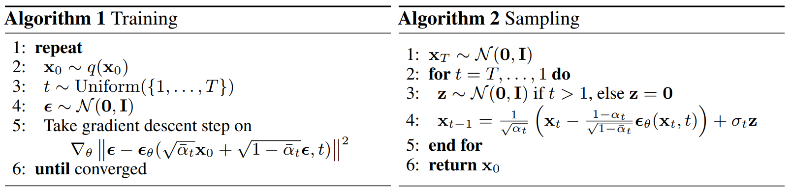
The sampling process (Algorithm 2) is similar to Langevin dynamics using $\epsilon_\theta$ as the learned gradient of the data density.
In addition, if $\mu_\theta$ with parameterization is substituted into the objective function expression,
\[\begin{equation} L_{t-1} - C = \mathbb{E}_{x_0, \epsilon} \bigg[ \frac{\beta_t^2}{2\sigma_t^2 \alpha_t (1-\bar{\alpha}_t )} \| \epsilon - \epsilon_\theta (\sqrt{\vphantom{1} \bar{\alpha}_t} + \sqrt{1-\bar{\alpha}_t} \epsilon, t) \|^2 \bigg] \end{equation}\], which is similar to denoising score matching at different noise levels and equals the variational bounds of the Langevin-like reverse process.
3. Data scaling, reverse process decoder, and $L_0$
Image data is given as an integer from 0 to 255 and linearly scaled as a real number from -1 to 1. This allows the reverse process to start with a standard normal prior $p(x_T)$ and always go to the scaled image. In order to obtain a discrete log likelihood, the last term L_0$ of the reverse process is computed as an independent variable from the Gaussian distribution $\mathcal{N} (x_0; \mu_\theta (x_1, 1), \sigma_1^2 I)$. is set as a discrete decoder.
\[\begin{aligned} p_\theta (x_0 | x_1) &= \prod_{i=1}^D \int_{\delta_{-} (x_0^i)}^{\delta_{+} (x_0^i)} \mathcal{N} (x; \mu_\theta^i (x_1, 1), \sigma_1^2) dx \\ \delta_{+} (x) &= \begin{cases} \infty & (x = 1) \\ x + \frac{1}{255} & (x < 1) \end{cases} \quad &\delta_{-} (x) = \begin{cases} -\infty & (x = -1) \\ x - \frac{1}{255} & (x > -1) \end{cases} \end{aligned}\]$D$ is the dimensionality of the data and $i$ represents each coordinate.
4. Simplified training objectives
The authors simplified the training objective as follows.
\[\begin{equation} L_{\rm{simple}} := \mathbb{E}_{t, x_0, \epsilon} \bigg[ \| \epsilon - \epsilon_\theta (\sqrt{\vphantom{1} \bar{\alpha}_t} + \sqrt{1-\bar{\alpha}_t} \epsilon, t) \|^2 \bigg] \end{equation}\]Here $t$ is uniform between 1 and T. Simplified objective is a form in which the weights are removed from the existing training objective. This weight term is a function of $t$, and since $t$ has a larger value as $t$ is smaller, a larger weight is given and learned when $t$ is small. That is, it is learned by focusing on removing noise from data with a very small amount of noise. Therefore, learning proceeds well in very small t$, but learning does not work well in large t$, so learning proceeds well even in large t$ by removing the weight term.
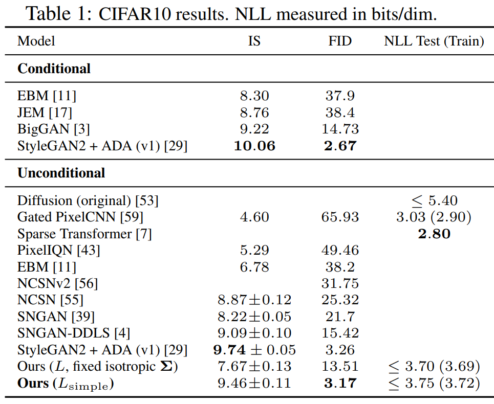
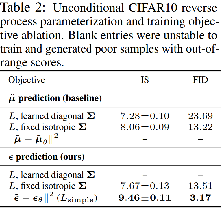
Through experiments, it was confirmed that $L_{\rm{simple}}$ with weight terms removed produced better samples.
Experiments
- $T = 1000$ in all experiments
- $\beta_t$ increases linearly from $\beta_1 = 10^{-4}$ to $\beta_T = 0.02$
- At $x_T$, the signal-to-noise-ratio is as small as possible $(L_T = D_{KL}(q(x_T\vert x_0) \; | \; \mathcal{N}(0,I)) \approx 10^{-5})$
- U-Net backbone using group normalization for neural network (similar structure to unmasked PixelCNN++)
- Input time $t$ to model with Transformer sinusoidal position embedding
- Use self-attention in 16x16 feature map
Results


![[Paper review] Self-correcting LLM-controlled Diffusion Models](/assets/images/blog/post-5.jpg)