


NeurIPS 2021. [Paper] [Github]
Zihang Dai, Hanxiao Liu, Quoc V. Le, Mingxing Tan
Google Research, Brain Team
9 Jun 2021
Introduction
Vision Transformer (ViT) shows similar performance to SOTA ConvNets among CNN-based models when trained on the JFT-300M dataset, which is a large-scale dataset. However, if you train only with ImageNet without additional training on a large-scale dataset, ConvNets lose performance at the same model size.
What can be seen from these results is
- Vanilla Transformer layer has higher capacity than CNN-based models.
- However, the generalization ability of CNN-based models is poor.
- To overcome this, a lot of data and computing resources are required.
The purpose of this paper is to improve accuracy and efficiency while effectively mixing the generalization of convolution and the capacity of attention.
The paper confirmed two facts:
- Depthwise convolution is effectively merged with the attention layer.
- High generalization and capacity can be obtained just by stacking convolution layers and attention layers in an appropriate way.
CoAtNet (Convolution + self-Attention) was created based on the above two facts.
Model
1. Merging Convolution and Self-Attention
The author paid attention to the MBConv block (used in MobileNetV2) that uses depthwise convolution, because both Feed Forward Network (FFN) of Transformer and MBConv use an inverted bottleneck structure. The inverted bottleneck structure expands the channel size of the input by a factor of 4 and then projects a 4x-wide hidden state to the original channel size to enable residual connection.
Due to the similarity of the inverted bottleneck, depthwise convolution and self-attention can be expressed as a per-dimension weighted sum of values of a predefined receptive field.
Depthwise convolution:
\[\begin{aligned} y_i = \sum_{j \in \mathcal{L} (i)} {w_{i-j} \odot x_j} \end{aligned}\]($x_i , y_i \in \mathbb{R}^D$ is the input and output in $i$, $\mathcal{L} (i)$ is the local neighborhood of $i$)
Self-attention:
\[\begin{aligned} y_i = \sum_{j \in \mathcal{G}} {\frac{\exp(x_i^T x_j)}{\sum_{k \in \mathcal{G}} \exp(x_i^T x_k)} x_j} = \sum_{j \in \mathcal{G}} {A_{i,j} x_j} \end{aligned}\]($\mathcal{G}$는 global spatial space)
The strengths and weaknesses of each operation are as follows.
- Input-adaptive Weighting Depthwise convolution kernel $w_{i-j}$ is an input-independent parameter, but attention weight $A_{i,j}$ is input-dependent. Therefore, self-attention is good at capturing the relationships between different locations, which is a necessary ability when dealing with high-level concepts. However, overfitting easily occurs when the data is limited.
- Translation Equivariance $w_{i-j}$ only considers the relative positions ${i-j}$ of the two points $i$ and $j$, but does not consider the absolute positions of each of $i$ and $j$. This feature improves generalization in datasets of limited size. On the other hand, ViT lacks generalization because it considers the absolute position using positional embedding.
- Global Recpetive Field The receptive field of self-attention is the entire image, but the receptive field of convoluton is small. When the receptive field is large, the model capacity increases because there is more contextual information. However, the complexity of the model increases and more calculations are required.
Therefore, the ideal model should have high generalization through translation equivariance and high capacity through input-adaptive weighting and global receptive field.
To combine the convolution equation and the self-attention equation, we simply added a global static convolution kernel and an adaptive attention matrix. At this time, there are two ways to add before (pre) or after (post) softmax normalization.
Pre-normalization:
\[\begin{aligned} y_i^{\text{pre}} = \sum_{j \in \mathcal{G}} {\frac{\exp(x_i^T x_j + w_{i-j})}{\sum_{k \in \mathcal{G}} \exp(x_i^T x_k + w_{i-k})} x_j} \end{aligned}\]Post-normalization:
\[\begin{aligned} y_i^{\text{post}} = \sum_{j \in \mathcal{G}} {\bigg( \frac{\exp(x_i^T x_j)}{\sum_{k \in \mathcal{G}} \exp(x_i^T x_k)} + w_{i-j}\bigg) x_j} \end{aligned}\]In the case of the pre-normalization version, the attention weight $A_{i,j}$ is determined by $w_{i-j}$ of the translation equivariance and $x_i^T x_j$ of the input-adaptive $x_i^T x_j$ of the translation equivariance, and both effects can be seen depending on the relative size. can Here, in order to enable global convolution kernel without increasing the number of parameters, scalar instead of vector $w_{i-j}$ Use $w \in \mathbb{R}^{O(|\mathcal{G}|)}$.
Another advantage of using the scalar $w$ is that the information for every ($i,j$) pair is included while computing the pairwise dot-product attention. Because of these advantages, pre-normalization is used instead of post-normalization.
2. Vertical Layout Design
Since the global context increases in proportion to the square of the spatial size, the calculation will be extremely slow if relative attention is applied directly to the input image. Thus, there are three options for realistic model implementation.
- After reducing the spatial size by down-sampling to some extent, global relative attention is used.
- By performing local attention, the attention of the global receptive field $\mathcal{G}$ is limited to the local field $\mathcal{L}$. → Non-trivial shape formatting operation of local attention requires excessive memory access.
- Replace quadratic softmax attention with a specific variant of linear attention. → I did a simple experiment and the result was not good.
Because of the above problems, the first method was chosen.
There are two major down-sampling methods.
- Use a convolution stem with a large stride as used in ViT (ex. stride 16x16)
- Using a multi-stage network with incremental pooling as used in ConvNets
Experiments were conducted on five models to find the best method.
- After using ViT’s convolution stem, a model in which $L$ Transformer blocks with relative attention are stacked → Marked as VITREL
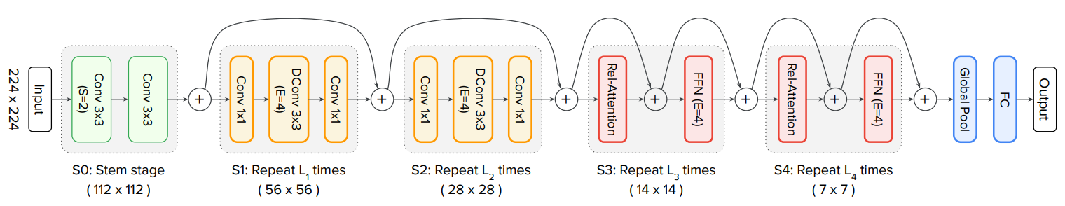
- It consists of 5 stages (S0 ~ S4) by imitating the structure of ConvNets. S0 is a 2-layer convolution stem. S1 is an MBConv block using squeeze-excitation (SE). S2 to S4 select between MBConv block and Transformer block. (Choose MBConv block to always go before Transformer block) → C-C-C-C, C-C-C-T, C-C-T-T, C-T-T-T (C is MBConv block, T is Transformer block)
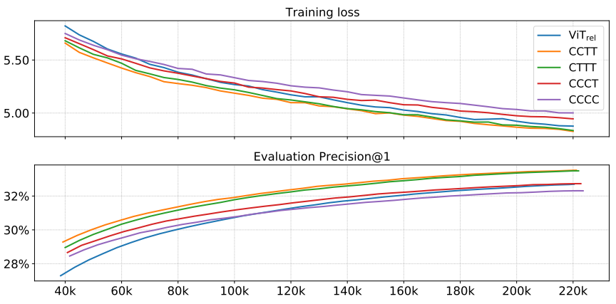
Generalization and model capacity were confirmed for 5 models.
Generalization: ImageNet-1K (1.3M) 300 epochs Check the difference between training loss and evaluation accuracy. If the training loss is the same, it can be said that the model with higher evaluation accuracy generalizes better.

Model capacity: JFT (300M) 3 epochs Measures how well a large training dataset works. If the final performance on a large training dataset is better, then the capacity of the model is high. As the size of the model increases, the capacity also increases, so the size of the five models was adjusted similarly and the experiment was conducted.
Transferability: A transferability test was conducted to determine a better model between C-C-T-T and C-T-T-T. Each JFT pre-trained model was finetune for 30 epochs on ImageNet-1K and then the performance was compared.
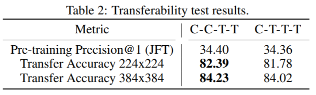
Finally, it was decided that C-C-T-T had better transfer performance.
3. Model structure
Experiments
- Experiment with 5 CoAtNet models of different sizes

- Dataset: ImageNet-1K (1.28 million images), ImageNet-21K (12.7 million images), JFT (300 million images)
- Pre-train: 300, 90, and 14 epochs with 224x224 images for each data set
- Finetune: 30 epochs with ImageNet-1K 224x224, 384x384, 512x512 images
- ImageNet-1K 224x224 is evaluated without a separate finetune (since it is the same dataset and the same image size anyway) -Data Augmentation: RandAugment, MixUP
- Regularization: stochastic depth, label smoothing, weight decay
Results
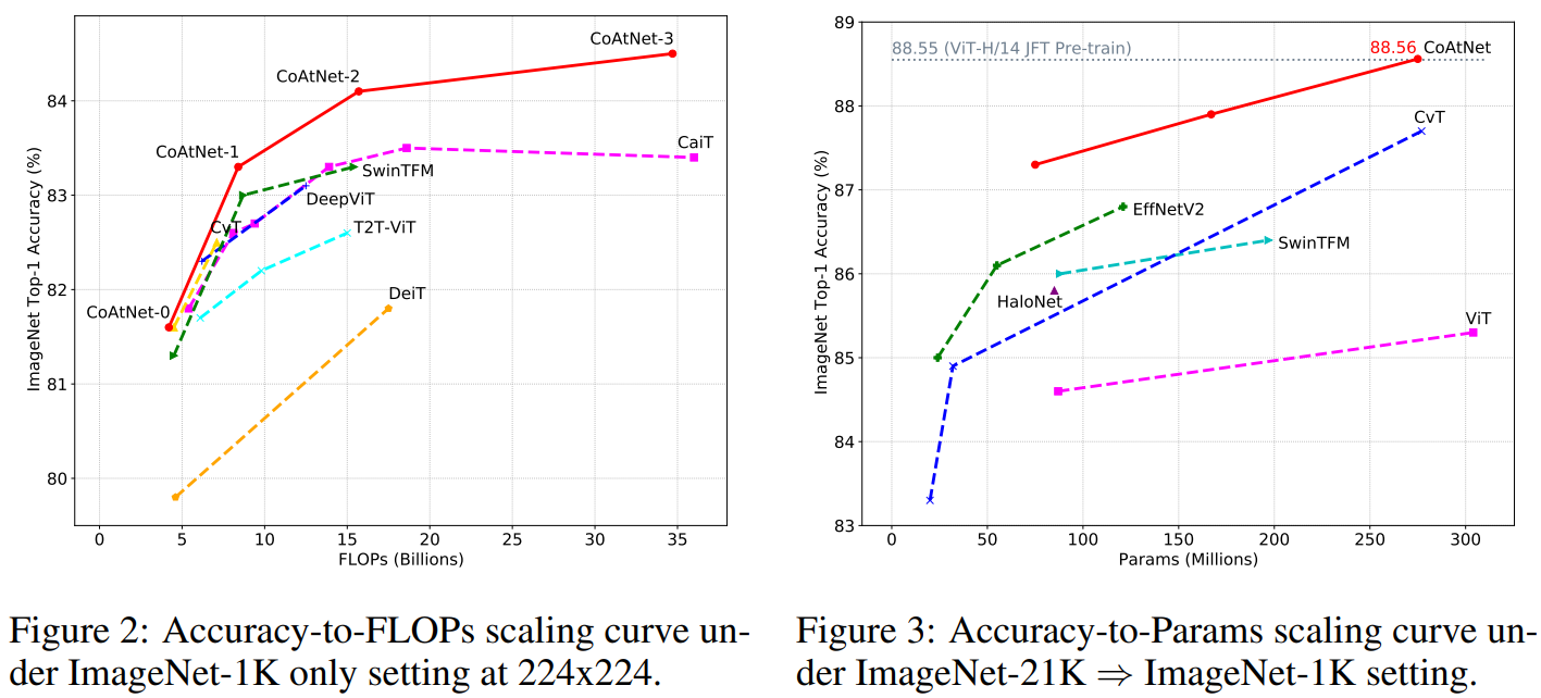
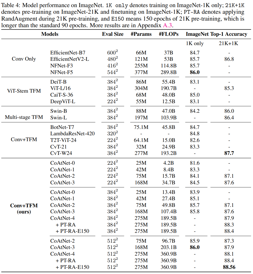
In addition, the size of the model was increased and compared with the existing model.
- CoAtNet-5: Setting as a training resource similar to NFNet-F4+
- CoAtNet-6/7: Setting as a training resource similar to ViT-G/14, learning with JFT-3B dataset.

- CoAtNet-6: Achieves 90.45% performance with 1.5 times fewer operations than ViT-G/14
- CoAtNet-7: top-1 accuray at 90.88% new state-of-the-art title
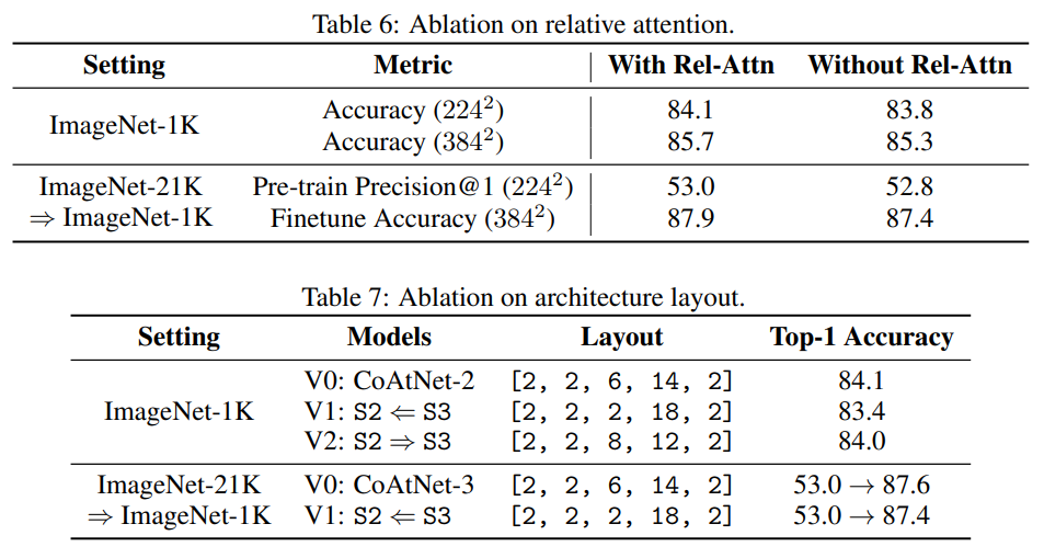
Ablation study
![[Paper review] Self-correcting LLM-controlled Diffusion Models](/assets/images/blog/post-5.jpg)